| ds2 = |
┌ 1 0 0 ┐ │ 0 1 0 │ └ 0 0 1 ┘ |
┌ x ┐ │ y │ └ z ┘ |
┌ x ┐ │ y │ └ z ┘ |
= |
┌ 1x+0y+0z ┐ │ 0x+1y+0z │ └ 0x+0y+1z ┘ |
┌ x ┐ │ y │ └ z ┘ |
= |
┌ x ┐ │ y │ └ z ┘ |
┌ x ┐ │ y │ └ z ┘ |
= | x2 + y2 + z2 | (equation 4) | |
| gμν = |
┌ 1 0 0 ┐ │ 0 1 0 │ └ 0 0 1 ┘ |
(equation 5) |
| gμν = |
┌ ∂x/∂x ∂x/∂y ∂x/∂z ┐ │ ∂y/∂x ∂y/∂y ∂y/∂z │ └ ∂z/∂x ∂z/∂y ∂z/∂z ┘ |
(equation 6) |
| A = |
┌ a11 a12 a13 ┐ │ a21 a22 a23 │ └ a31 a32 a33 ┘ |
(equation 7) |
| V = |
┌ v1 ┐ │ v2 │ │ v3 │ └ v4 ┘ |
| aij | = |
∂xi ---- (equation 12) ∂xj |
| x'i | = | Σ |
∂x'i ---- xj (equation 13) ∂xj |
|
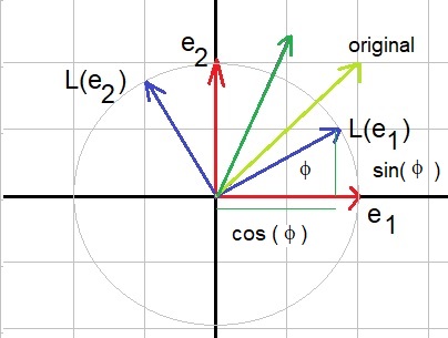
┌ cos(ϕ) -sin(ϕ) ┐ └ sin(ϕ) cos(ϕ.) ┘ |
|
┌ x1' ┐ └ x2' ┘ |
= |
┌ cos(ϕ) -sin(ϕ) ┐ └ sin(ϕ) cos(ϕ.) ┘ |
┌ x1 ┐ └ x2 ┘ |
| A'i | = | Σ |
∂x'i ---- Aj (equation 16) ∂xj |
| A'i | = | Σ |
∂xj ---- Aj (equation 17) ∂x'i |
|
┌ 1 0 0 ┐ │ 0 1 0 │ └ 0 0 1 ┘ |
|
┌ -xy -y2 ┐ └ x2 xy ┘ |
| A'ij | = | Σ Σ |
∂x'i ∂x'j ----------- Akl (equation 18) ∂xk∂xl |
| C'ij | = | Σ Σ |
∂xk ∂xl ----------- Ckl (equation 19) ∂x'i∂x'j |
| ds2 = |
┌ -1 0 0 0 ┐ │ 0 1 0 0 │ │ 0 0 1 0 │ └ 0 0 0 1 ┘ |
┌ ct ┐ │ x │ │ y │ └ z ┘ |
┌ ct ┐ │ x │ │ y │ └ z ┘ |
= |
┌ -ct+0x+0y+0z ┐ │ 0ct+1x+0y+0z │ │ 0ct+0x+1y+0z │ └ 0ct+0x+0y+1z ┘ |
┌ ct ┐ │ x │ │ y │ └ z ┘ |
= |
┌ -ct┐ │ x │ │ y │ └ z ┘ |
┌ ct ┐ │ x │ │ y │ └ z ┘ |
= | -c2 t2 + x2 + y2 + z2 | ||
| c2 | = |
1 ---- ε0 μ0 |
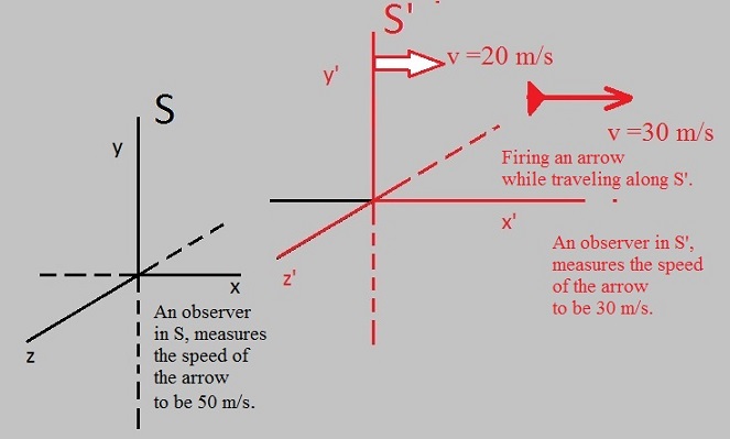
| x' | = | x-vt ------------- √(1-v2/c2) |
| y' | = | y |
| z' | = | z |
| t' | = | t - (v/c2).x ------------- √(1-v2/c2) |
| γ | = | 1 ------------- √(1-v2/c2) |
| x' | = | γ | (x-vt) |
| y' | = | y |
| z' | = | z |
| t' | = | γ | (t - (v/c2).x) |
| ds2 = |
┌ -1 0 0 0 ┐ │ 0 1 0 0 │ │ 0 0 1 0 │ └ 0 0 0 1 ┘ |
┌ ct ┐ │ x │ │ y │ └ z ┘ |
┌ ct ┐ │ x │ │ y │ └ z ┘ |
= |
┌ -ct+0x+0y+0z ┐ │ 0ct+1x+0y+0z │ │ 0ct+0x+1y+0z │ └ 0ct+0x+0y+1z ┘ |
┌ ct ┐ │ x │ │ y │ └ z ┘ |
= |
┌ -ct┐ │ x │ │ y │ └ z ┘ |
┌ ct ┐ │ x │ │ y │ └ z ┘ |
= | -c2 t2 + x2 + y2 + z2 | ||
|
┌ g11 g12 g13 g14 ┐ │ g21 g22 g23 g24 │ │ g31 g32 g33 g34 │ └ g41 g42 g43 g44 ┘ |
|
┌ g11 g12 g13 g14 ω15 ┐ │ g21 g22 g23 g24 ω25 │ │ g31 g32 g33 g34 ω35 │ │ g41 g42 g43 g44 ω45 │ └ ω51 ω52 ω53 ω54 ω55 ┘ |
| gμν = |
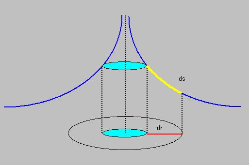
┌ -(1-R/r) 0 0 0 ┐ │ 0 1/(1-R/r) 0 0 │ │ 0 0 r2 0 │ └ 0 0 0 r2sin2(θ) ┘ |