Basic notes on IT.
In the series: Note 13.
Subject: Quick introduction DWH and OLAP Technologies.
Date : 25 October, 2016
Version: 0.1
By: Albert van der Sel
Doc. Number: Note 13.
For who: for beginners.
Remark: Please refresh the page to see any updates.
Status: Ready.
Contents:
1. Background, and Datawarehouse (DWH) Technologies.
1.1 Data Warehouse technology and terms.
1.2 OLAP and Cubes.
1.3 A few words on ETL.
2. A few notes and preliminaries before using Visual Studio (or BIDS) for building a Cube.
2.1 Create a fact- and dimension tables and loading some data.
2.2 Relation between Visual Studio (or "BIDS"), and SSAS.
3. Building and deploying a Cube.
Chapter 1 is a fast introduction in Data Warehouse (DWH) terms and technologies (like dimensions, cubes etc..).
So this chapter is quite "generic" and can be used by anyone who is interested in DWH.
Chapters 2 and 3 are more geared towards using "SQL Server Analysis Server", which enables us
to implement OLAP technologies with cubes and other objects.
If you want a quick and simple intro in "SQL Server Analysis Services (SSAS)", you best read all 3 chapters.
If you want some simple information on DWH with OLAP/Cubes, then only chapter 1 should be enough.
1. Background, and Datawarehouse (DWH) Technologies.
This is an very simple and short intro in DWH Technology.
Here I presume that you know SQL Server, or any other RDBMS like Oracle, reasonably well.
So, you "know your way" with tables and indexes, and you (for example) know what Primary keys and Foreign keys are used for.
This note is involved with:
- Data Warehousing,
- Business Intelligence,
- OLAP and cubes, and
- Data Mining.
Let's first spend a few words on the above terms, which are all interrelated.
1.1 Data Warehouse (DWH) technology and terms:
The usual databases you find in the business, are "transactional" oriented (OLTP), meaning they are optimised for quickly storing (and retrieving) individual
transactions, but they are usually not used or suited for storing all sorts of "aggregates" or "summarized data" and analysis.
In such OLTP database, most queries which are specifically designed for analysis or summaries, often use many "nested joins"
which may severely impact the performance of that database.
What's more, many companies have not just one, but usually a number of databases. In such a setup, it's not easy to find
answers that many analists (and folks like marketeers) are looking for. They want to analyze "trends" and "mine" data
to find answers that might be sort of "hidden" in the bulk of all those individual databases together.
One path that's often been followed, is to create one special database, the DWH, containing specifically crafted tables, that gets
loaded with data from all other relevant databases.
So, you might imagine that the company has one large Oracle transactional database, with a variety of other database (which
could be a mix of Oracle, or SQL Server or whatever other type of RDBMS). Let's call that "bunch" of source data, "the primary sources".
Now, the "developers & DBA & analists" have to work together to create the DWH, and make sure it gets properly loaded
from all those primary sources.
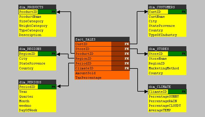
The tables in the DWH, are usually one or more "fact tables" and a number of "dimension tables".
Let's assume we have just one fact table, and a small number of dimension tables (like 5 or 6 or so).
What exactly the fact- and dimension tables represent, will be discussed below.
Here we arrive to the true heart of the DWH.
Fig 1.
The fact table:
We know that all of the data of the primary sources, are all facts. As an example, let's suppose that there 5 primary
source databases. We cannot expect that the "layout" of all tables over all those databases, are the same.
Indeed. We can expect that there are quite some differences between the core tables in those 5 primary source databases.
The "developers/DBA/analists" will study this matter, and do their best to create a fact table in the DWH,
with such chosen columns, that it best represents the overall data/facts. This means that for example, one source database might
store data of "orders", another source database carry all sorts of facts of customers (maybe from some ERP database), while
another source database carries all sorts of facts about products, while another database stores facts of Regions and another
about repairs at customers, etc.. etc..
So, the "developers/DBA/analists" will create the fact table in the DWH in such a way, that it will have the most interesting columns
from those tables in the sources.
Ofcourse, there might exist relatively simple fact tables, but usually it's quite a challenge to design one.
For one thing: you need to know "the business" quit well !
Also, you can imaging that it could be quite some challenge too, to load this fact table with data from the sources.
The dimension tables:
Suppose you have one fact table, called "fact_SALES", containing all sorts of facts around the sales of a company.
So it is a large bunch of records, pure data, listing for example ProductID's, StoreID's, RegionID's, PeriodID's, AmountSold, Revenues etc..
The dimension tables, usually below 10 or so, will all individually focus on "one dimension". You know that generally
speaking, a "dimension" is something along which you want to "measure" something. For example, to fix a position in space,
you can measure it along the x-, y- and z dimensions. Now, in DWH thechnology it works quite the same way.
For example, if we would indeed have a SALES fact table, we might have a "product" dimension table which describes
the products. And we might have a "regions" table, which describes all the characteristics of the different regions where our Stores are located.
The point is, that you can design queries that joins the fact table with one (or more) dimensions, which let's you 'measure"
the facts along those dimensions. For example: you can focus on AmountSold and Revenues (from the fact table) "measured" along Regions,
where all the Regions are stored in a dimension table (for example the dim_REGIONS table).
What starts to unfold, is a "star-like" schema, where the fact table is in the centre, while the dimension tables
are located all around the fact table.
The crux of the story will get clear soon. Let's first take a look at the "star-like" schema shown in figure 1.br>
It's neccessary that the "fact table" uses Foreign Keys, which all points to Primary Keys in the "dimension tables".
The dimension tables, which usually are much smaller than the fact table, are normalized in the sense that they
contain unique records. So, for example, the "dim_CUSTOMERS" table, will list all customers, while every record in that table
is "unique" (garanteed by the Primary Key). So, it simply just lists all customers.
In a "query", the fact table (which might contain many records), can be "joined" to one or more dimension table(s),
using the PK-FK relation(s), which should enhance performance.
Indeed, using the star-like schema, also the number of joins can be kept to a minimum, as compared to the usual joins used in an OLTP database.
This already justifies the use of a DWH:
- You have consolidated data from multiple sources and databases in one DWH. Thats very good for business analysis.
- You have off-loaded, or seperated, "analysis" from your regular OLTP databases.
- In general, the DWH is better optimized for queries (e.g.: less joins needed)
Some drawbacks exists too, for example:
- Additional resources must be available like cpu power and Storage, which could be very significant.
- Additional support and manpower is needed which can vary between "some light work", to a whole department involved with the DWH.
- In some cases: A DWH "lives" and it never seems to get quite finished.
The "entity relationship" shown in figure 1, is indeed called a "star schema". An extension to this is popular too. This extension
is called a "snowflake schema". Here too, we have dimension tables linked directly to the fact table, but there are also
one or more dimension tables (at the "fringes") which are linked to first dimension tables, but not to the fact table.
But for our discussion it's not really a fundamental difference.
Note 1:
Also be aware of the fact that next to the fact/dimension tables, additional tables may live in the DWH which carry all sorts of aggregated
information. This is often done to "pre-calculate" all sorts of summations and averages, so that information can be queried quickly.
Note 2:
Figure 1 tries to display an implementation using facts/dimension tables, which is a popular and effective way to
implement a model for a DWH. However, alternatives exists, and even non-relational alternatives exists.
Measures:
If you take a look again at the fact table in figure 1, then you see a lot of Foreign Keys (pointing to the Primary Keys of the dim tables).
But the fact table usually has more columns, listing facts. These are not foreign keys. Actually, this is important data
where analysts are most interested in. This sort of columns in the fact table, are called the "measures".
Formally, measures are often defined as those columns in the fact table, on which aggregations and the like can be performed,
like sum(), avg() and that kind of stuff. If we follow that definition, the "AmountSold" in the fact table, would be a true "measure".
However, be aware of the fact that in many DWH docs, every non-FK column in a fact table, might be called "a measure".
Hopefully you can see interesting scenario's. For example, you might join the "fact_SALES" table with the "dim_REGIONS" table,
while in that query, you "group" by StateProvence and you also "summarize" on the AmountSold.
This quickly leads to insight where, viewed from geographical perspective, the subtotals of AmountSold values are high and low.
Hierarchies in dimensions:
Note that for some Dimension tables, a certain hierarchy might be present. For example, in the dim_PERIODS table, we can see
for example the year, quarter, and month columns. Now, we know that "a year" contains 4 quarters, and that a year spans 12 months.
Using smart queries, or Business Intelligence tools, the hierarchy present in certain columns, makes it easy to "drill down",
or the other way, "roll up" along such an element in the hierarchy. It means that you then switch the view from "detail" to "summary".
Ofcourse, not all dimension tables need to have such an hierarchy implemented "perse".
Loading a DWH:
Due to the fact that the source databases change over time, the DWH needs to be "refreshed" periodically as well.
For many businesses, once a week (or maybe once every night), the DWH will be refreshed.
In many cases, it means that all tables gets truncated and will reloaded from the source databases.
As said before, this will be often done in a weekly (or nightly) batch.
However, if a DWH is really very large, the refresh is quite some operation, and the periodicity might be lowered substantially.
So, a "Full Reload" is then often "too wild..." (takes too much time, takes too much performance etc...)
In general, people distinguish between a "Full Load/Refresh" where the DWH is actually (almost) completely "reloaded",
and "Incremental Loads" where only new and altered data is loaded.
Indeed, in many scenario's a Full Reload only happens with a very low freqency, while an Incremental Load happens
with a higher freqency, like once every night.
In some cases, "real time" links from the source databases to the DWH are implemented, meaning that
changes in the (operational) OLTP databases will be refelected (near-realtime) in the DWH as well.
But this in not seen very often. One example implementation could be the use of CDC and streams in Oracle.
However, most often, the refresh is just arranged by a nightly batch, also done in order to minimize the burden on
the operational OLTP databases.
The loadprocess itself could range from "fairly simple" to "pretty tough", all depending on the size and complexity.
By the way, it is important to realize that, once loaded, the DWH is used mainly for "read-only", that is using SELECT queries,
and usually no updates and inserts takes place.
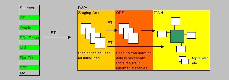
In many implementations, the DWH actually consists of three parts: A staging area (where staging tables live),
and an Operational DataStore (ODS), and then the actual DWH where the facts and dimensions live.
In such a model, some jobs will load the Staging tables first. Then, if the data in the Staging tables
needs to be processed/transformed further before it's usable, other scripts and jobs might "massage" (or "transform")
the data and store it in the ODS.
Then, the final round might be that the data in the ODS gets loaded into the "real" DWH.
Not in all cases an ODS is needed. Some DWH implementations only use Staging tables for the initial load,
while other jobs see to it, that the true DWH gets loaded.
Ofcourse, in a really simple DWH environment, it might be so, that even the use of Staging area is unneccessary.
It just depends on the complexity of the load/transformation actions.
The loading and transforming of data, falls under the concept of "ETL", which is short for Extracting, Transformation, and Loading.
Up to now, we considered that the DWH is build from other operational OLTP databases. But in reality the sources could be "very"
divers, like for example: Databases, flat files, Office documents, XML documents etc.. etc..
Indeed: that's a complex variety of "sources". Needless to say that the ETL processes involved, might be quite complex too.
In the Microsoft "world", ETL is often implemented using socalled "SSIS" packages.
The whole "suite" of Microsoft SQL Server 2005/2008/2012 "Business Intelligence" (BI) tools are formed mainly by three products:
- SSAS (SQL Server Analysis Services) is the subject of this note, so we will see more of this environment later on. It's mainly involved with socalled "cubes".
- SSIS (SQL Server Integration Services) enables you to perform ETL from various sources, into various destinations like a SQL Server based DWH.
- SSRS (SQL Server Reporting Services) enables you to create "Reports" from various datasources, of which a DWH could be an excellent source for reporting.
In SQL Server 2012, the three products still form the "core" of BI, but quite relevant additions were made.
For example, in 2012, we have better integration with Powerpivot, and more ways to "clean" data with ETL. Also, support
was added for the "opensource" product "Hadoop".
Apart from Microsoft, many third-party vendors deliver BI tools too, ranging from fairly simple products to quite complex environments.
The figure below depicts a birds-eye view of the processes and area's that might be involved in a (more or less) typical DWH environment.
Fig 2.
Note:
Not all DWH's are designed with a Staging area, ODS, DWH area etc.., or use a "Star/Snowflake" model of fact- and dimension tables.
Some more or less "ad hoc / sloppy" DWH's "just" use some tables, which resembles "fact tables",
and there are a number of pre-populated aggregate tables.
A number of scripts (or other processes) maintain those tables (like incremental loads), and with some Reporting Tool,
pre-defined "Reports" are available for users. It might just work..., just depending on the type of business and other factors.
1.2 OLAP and Cubes:
What's a cube?:
Here we are going discuss OLAP and cubes.
OLAP is short for "OnLine Analytical Processing". It is the collection of methods to design and create a "cube",
then "populating" (or calculating) the cube, and from there on, perform "multi-dimensional" analysis of the data in the cube.
OK, but what is a cube then?
A star schema, or snowflake schema, of a fact table and dimensional tables in a DWH, as we have discussed in section 1.2, can serve
as a basis for creating a cube.
A "cube" is an object which which has no real equivalent in Relational Database technology. The object is multi-demensional
(analog to a 3D cube), and is created by the OLAP software. In our case, the OLAP engine is SSAS.
Here is a plausible description of a cube: if you would "fold" the dimension tables of the starschema around the facttable,
something is going to get into existence, that "looks" like a cube. Now just imaginge that the measures (2D sheet) in the "fact_SALES" are
positioned horizontally (on the floor so to speak), and the "dim_PERIODS" dimension table is fold vertically, we get a 3D object.
It will be the floor and one side of a cube.
Now the trick is: the OLAP software will calculate all aggregates of a measure (like AmountSold) over all values of the dimension.
In this case, since our example deals with the dim_PERIODS dimension, we get AmountSold with respect to the years, AmountSold over
all months, AmountSold over all weeks in a month.
The same is done with respect to any other Dimension you have added to the cube.
Now the remarkable thing is: the cube "knows" the answers to all posible queries already in advance. Every summation, or average etc..
is already calculated (!) and stored in the cube.
Now, if a fact table is very large (many rows) and has quite a few Measures (the columns), "calculating" the cube, or what is also often said,
"populating" the cube, might take quite a while (for example: a few hours or so, or even longer).
The advantage is: you can let the OLAP software calculate (populate) a large cube at night, and the next morning it might be ready
for querying by your analists.
The great advantage of a cube is that all results are pre-calculated, and thus response time should be orders of magnitude
better compared to a regular Relational model.
You get it? If yes, you are there!
The rest, like using tools to create and maintain a cube etc.. is just "mechanics".
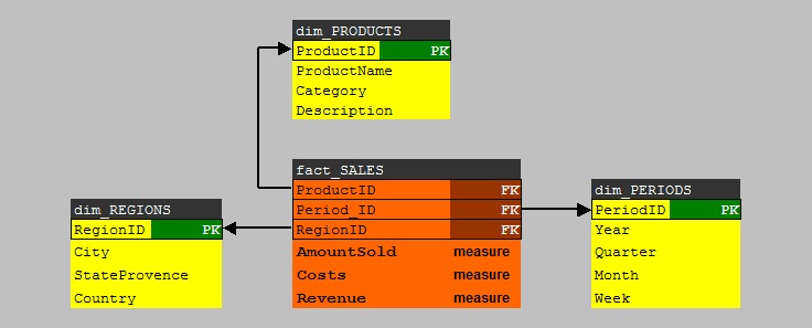
Let's study a very simple example. Lets take a look at starschema using a "fact_SALES" fact table, and using three dimensions,
namely "dim_PERIODS", "dim_REGIONS", and "dim_PRODUCTS". See figure 3 below:
Fig 3.
Although it's a very simple starschema, we can build a "cube" from this model.
Note that the fact table has 3 important "measures": AmountSold, Costs, and Revenue. Analysts are usually most interested
in those numbers, especially if they can easily map it to Regions and Periods. That's information !
Note that the dim_REGIONS and dim_PERIODS dimension tables, have a hierarchy implemented:
- YEAR contains QUARTERS which contains MONTHS.
- COUNTRY contains STATEPROVENCE which contains CITIES.
You can almost see it happen when you build and populate the cube.
For example, we can let the OLAP engine calculate grand totals of AmountSold, Costs, and Revenues per Country/Year,
and the OLAP engine will calculate all "childs" below the parents (country/year), so, the cuble will also store
AmountSold, Costs, and Revenues per Month/City etc.. etc..
This information will be available directly, once the cube is fully build (fully populated).
Marketeers and other analysts will get their numbers very quickly.
Using the right BI tools, they can "roll up" numbers to get summarized data, or "drill down" to childs to get detailed numbers.
MDX Queries:
You know that with the "usual SQL", you can query the regular (2 dimensional) tables in an ordinay database (like a DWH or OLTP database).
Standard SQL is already a great tool, also for creating fantastic reports with all sorts of summaries, by just querying ordinary tables.
For example, you can use functions in the SELECT statement (like sum(), avg() etc..), and used in conjunction with GROUP BY and ROLLUP and other clauses,
much power is in your hand. But this is to be used for regular databases.
So how can you retrieve data from a cube?
- Several BI tools makes that possible.
- Combining SSAS with SharePoint 2010 is a promising path to follow.
- Some Office components (Excel 2010, webcomponents) allows it too.
- Or you write MDX queries.
MDX is short for "Multidimensional Expressions", and MDX queries makes it possible to SELECT data from multidimensional datasets like a cube.
So, even from a SQL prompt, it's possible to query a cube, although the statements are a "tiny" bit "tougher" than the usual SQL you
use to query regular tables.
This is due to the fact that you must navigate in multiple dimensions, instead of only rows and columns, and that fact will be relfected
in the syntax.
In it's basic form, the MDX statement looks familiar, because it is in the usual form "SELECT .. WHERE .. FROM (cubename)".
However, since you navigate along certain "axes" in the cube, you specify those with the "ON COLUMNS" and "ON ROWS" keywords.
In principle, the resultset could be multidimensional too. However, most reports will be in the traditional 2 dimensional form,
(since we humans are so accustomed to that) so many MDX queries traverse one choosen dimension for the "ON COLUMNS", while the datarows
will be the "measures" of interest, specified by the "ON ROWS".
Here is a very simple example:
SELECT {[dim_REGIONS].[City]} ON COLUMNS,
{[measures].[AmountSold]} ON ROWS
FROM [MyCube]
1.3 A few words on ETL:
ETL is centered around:
- "Extracting", meaning how to get data from a source system,
- "Transforming", meaning do we need to "massage" or modify data, and
- "Loading", meaning how to get data into the target database.
Sources of data can be anything.
Usually, your DWH is build on an Oracle database, or SQL Server database,
or any other professional type of RDBMS. So that's usually the target type of database.
The sources however, can be of multiple types, like tabledata from other database systems, or flat files,
XML files, Office documents etc..
Many third-party tools (BI tools) exists, which can materialize this sort of jobs, and often you are able to
schedule them too (from e.g. the native job-agent belonging to the RDBMS, or the OS, or other sort of scheduling).
But the RDBMS itself usually has lots of facilities too, for example "prompt tools", but GUI like too.
This is certainly true for, for example, Oracle and SQL Server.
If you really would go (or maybe you are already) "in-depth" in those Oracle tools, the parallel options
are absolutely great.
For SQL Server, you might explore the native tools:
-bcp (OS prompt tool).
-TSQL scripts
-BULK INSERT tsql statement
-Import/Export Wizard
-SSIS
For Oracle, you might explore the native tools:
-sqlloader (OS prompt tool)
-impdp/expdp (OS prompt tools)
. transportable tablespace using impdp/expdp
. export or import of a full schema using impdp/expdp
- external table facility
- DBMS packages (plsql)
- OEM/Enterprise Manager
- further plsql options
2. A few notes before using Visual Studio or BIDS for building a Cube.
2.1 Create a fact- and dimension tables and load some data.
Our goal is to build a cube. It will be based on a simple starschema. So, we need some actual tables with some data.
Thus we need to do that first. In this section, you are encourage to load and execute a script that will create
a fact table and three dimension tables (just like was shown in figure 3).
I hope you have some SQL Server test system lying around somewhere. In the instance, create a database called "TEST" (or use some other name).
From the Management Console, start a Query Window, and make this TEST database your current database.
Copy and paste the following script in your Query Window, and execute it.
The script will only create the tables, and load some sample data in them.
-- 1. CREATE TABLES:
-- -----------------
create table dimREGIONS
(
RegionID int not null PRIMARY KEY,
City varchar(64) not null,
StateProvence varchar(64) not null,
Country varchar(64) not null
)
GO
create table dimPERIODS
(
PeriodID int not null PRIMARY KEY,
Year smallint not null,
Quarter smallint not null,
Month varchar(32) not null,
)
GO
create table dimPRODUCTS
(
ProductID int not null PRIMARY KEY,
ProductName varchar(64) not null,
Catagory varchar(64) not null,
Description varchar(64) null
)
GO
create table factSALES
(
ProductID int FOREIGN KEY references dimPRODUCTS(ProductID),
PeriodID int FOREIGN KEY references dimPERIODS(PeriodID),
RegionID int FOREIGN KEY references dimREGIONS(RegionID),
AmountSold int,
Costs decimal(7,2),
Revenues decimal(7,2)
)
GO
-- 2. LOAD TABLES:
-- ---------------
-- load dimREGIONS
insert into dimREGIONS values (1,'Amsterdam','NH','Netherlands')
insert into dimREGIONS values (2,'Alkmaar','NH','Netherlands')
insert into dimREGIONS values (3,'Rotterdam','ZH','Netherlands')
insert into dimREGIONS values (4,'Utrecht','UT','Netherlands')
insert into dimREGIONS values (5,'New York','NY','USA')
insert into dimREGIONS values (6,'Washington','DC','USA')
GO
-- load dimPERIODS
insert into dimPERIODS values (1,2008,1,'januari')
insert into dimPERIODS values (2,2008,1,'februari')
insert into dimPERIODS values (3,2008,1,'march')
insert into dimPERIODS values (4,2008,2,'april')
insert into dimPERIODS values (5,2008,2,'may')
insert into dimPERIODS values (6,2008,2,'june')
GO
-- load dimPRODUCTS
insert into dimPRODUCTS values (1,'Mountainbike','Bikes','Specifically designed for offroad')
insert into dimPRODUCTS values (2,'Citybike','Bikes','Specifically designed for use in cities')
insert into dimPRODUCTS values (3,'Racingbike','Bikes','Specifically designed for speed')
insert into dimPRODUCTS values (4,'Rollerskates','Skates','Specifically designed to break legs')
GO
-- load factSALES
insert into factSALES values (1,1,1,55,200.80,3000)
insert into factSALES values (1,3,1,7,99,5000)
insert into factSALES values (2,2,3,9,150,2000)
insert into factSALES values (2,5,5,95,8000,16000)
insert into factSALES values (2,2,3,23,1900,6000)
insert into factSALES values (2,6,4,28,1150,2000)
insert into factSALES values (4,3,1,12,900,5000)
insert into factSALES values (1,2,4,120,9000,50000)
insert into factSALES values (3,3,1,2,100,1000)
insert into factSALES values (4,2,4,70,9000,50000)
insert into factSALES values (2,1,5,95,1100,33000)
insert into factSALES values (2,2,5,65,900,14000)
insert into factSALES values (2,3,5,75,1900,15000)
insert into factSALES values (3,3,5,29,450,4700)
insert into factSALES values (3,1,5,11,650,2750)
insert into factSALES values (4,6,1,135,1150,4750)
insert into factSALES values (4,5,1,119,1050,4210)
insert into factSALES values (3,2,1,22,150,1250)
GO
Exercise:
As an exercise, you probably want to view a nice graphical datamodel of your DWH.
Well, that's certainly possible.
In the Management Console, click the "+" symbol that you see in front of the TEST database.
This container will fold open, and you probably will see the "Database Diagram" as the first sub-item.
Right-click the "Database Diagram" and choose "New Database Diagram". It is easy to follow the steps that will follow.
The result will be a nice graphical "Entity Relationship Diagram" of your four tables.
Now that we have a DWH with tables and data, we can play, and we will create a cube in Chapter 3.
2.2 Relation between Visual Studio (or "Business Intelligence Designer Studio"), and SSAS.
On the one hand, we have a SQL Server database, which is our DWH (the fact table and dimension tables).
A (multidimensional) cube is something like an external entity, actually considered to be "loose" from your DWH.
Connections to the DWH exists only when you populate it with data (there exists some exceptions).
Once loaded, the cube is again disconnected from the DWH, until the next refresh (the next re-population).
You might have two questions now.
⇒ How does one create a cube from the tables in a DWH?
⇒ Where is a cube stored?
You create a cube using "Visual Studio", or "Business Intelligence Designer Studio" (BIDS),
which both are pretty much the same thing.
Once you have build the cube, then you "deploy" it, meaning that metadata gets registered with the SSAS service.
You probably know, that with SQL Server Management Studio, you not only can connect to a Database Engine, but to SSAS too.
If a cube was indeed deployed using BIDS or Visual Studio, then in SQL Server Management Studio (and connected to SSAS),
you can see all properties of the cube, like which fact table and dimensions it contains, and many other properties.
Also, when connected to SSAS, you can also lauch MDX queries using a Query Window.
But a (molap) cube will not be stored in a SQL Server database.
About the actual physical storage of a cube, it depends a bit on the "OLAP" model used (MOLAP,ROLAP etc..)
when cube is designed. For example in the MOLAP case, it will be stored on disk, perhaps in multiple "partitions".
So, here the cube is not stored in the database. It will often use a "proprierty" storage structure on disk(s).
However, there are several OLAP models in use, for example:
- MOLAP is short for "Multidimensional" OLAP, and it's the model which is traditionally used for what
we usually understand to be a (multidimensional) "cube". This is the model we study in this note.
- ROLAP is short for "Relational" OLAP. It may come to you as a surprise, but the starschema's already shown
in this document (and created by the script of 2.1), actually are (simple) ROLAP implementations.
So, with ROLAP, we formally do not have an external "cube", although some Vendors like Microsoft let's you
create a cube, while the "relational" part of ROLAP refers to the storage/caching model (which uses the DWH).
So with ROLAP, we do not have such a multidimensional cube, as we do have with MOLAP.
- HOLAP. Some hybrids forms exists as well.
In this note, we will use MOLAP, which also means that we create and study Multidimensional cubes.
In such a case, it's not stored in a SQL Server database, except for some metadata.
The storage model is filebased with a proprierty structure. If it is anticipated that a cube would become very large,
you could define "measure groups" which might be stored on different disks.
3. Building and Deploying a cube.
This section will show you a few screendumps of using Visual Studio (or BIDS) on how to build and deploy a cube.
It's not very hard to do, once you have a starschema which forms the basis for a (molap) cube.
Remember, you design a cube using a client tool like Visual Studio (or BIDS), but once you deploy the cube,
only then you actually will register the metadata with the SSAS service.
From then on, you can "see" it too from the "SQL Server Management Console" (SSMS), if you are connected to SSAS.
Then, you could use it from Sharepoint, or use Excel, or use MDX queries from the Management Console etc.. etc..
So, deploying a cube, is like "making it alive for access" (under the control of SSAS).
You still need to populate the cube, but access control goes through SSAS.
The next step then would be to calculate or "populate" the cube, at which process the cube gets loaded with data and
parent and child aggregates are calculated (see chapter 1).
The population of the cube is a seperate step, which can be repeated later at any time.
In most cases, the cube is only "connected" to the DWH, when it gets populated. At all other times, it is just disconnected.
Step 1: Creating a "Multidimensional" project in Visual Studio:
If using SQL Server 2005/2008, you may find the "Business Intelligence Designer Studio" in your Start Menu.
With SQL Server 2012, it's possible that you only see "Visual Studio", but both tools are actually quite the same thing.
Start up Visual Studio, click File, click New, choose "Project".
Since we want a molap cube, in the following dialog box, choose "Analysis Service Multidimensional and DataMining".
Fig 4.
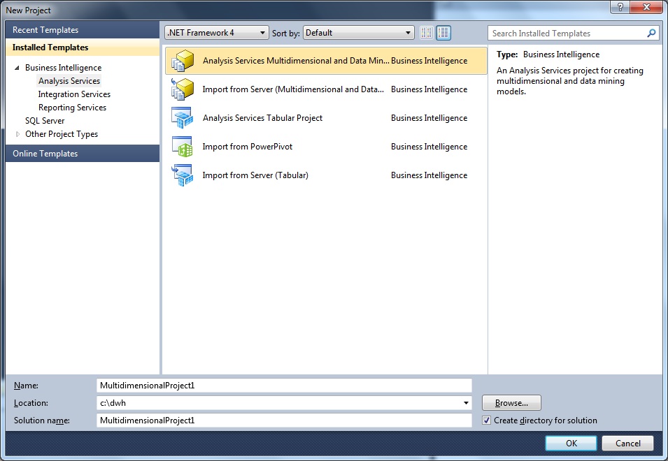
Note that I store the project in "c:\dwh". You might choose a similar location.
Step 2: Creating a "Datasource":
After step1, Visual Studio will show you several "sections" on your screen. Note the "Solution Explorer" (per default on the right side).
First we will create a "Datasource" which is not much more than creating a "connect string" to the DWH.
This is logical: your project "needs to know" to which SQL Server instance, and to which database, it should connect.
So rightclick the "Datasources" container, and choose "New Datasource"
Fig 5.
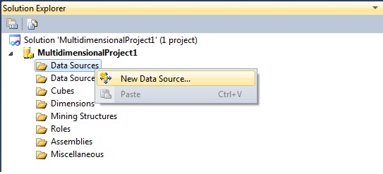
Next, the "New Datasource Wizard" will popup. Essentially you will next see a couple of Dialogboxes where you
have to select a Server instance, and a database, and which credentials for the connection should be used.
I skip those dialogboxes, because it's likely you have seen similar dialogboxes before. It's quite simple anyway.
Give the Datasource a name like "Test" (or some other name you like).
However, there might be one small optional "hurdle" to take, which is the "select impersonation information".
Here you can choose from several credentials which your project will use when you deploy it.
If, at the final step, the deploy goes wrong, it could well be due to your choice of the account used (insufficient permissions).
Step 3: Creating a "Datasource View":
Once the "Datasource" has be set, now we can choose the objects (fact and dimensions) which will form the basis of our cube.
For this, rightclick "Datasource Views" and choose "New Datasource View".
The "New Datasource View Wizard" will startup. First, select a "Datasource". This will be the Datasource as was created in Step 2.
The next screen allows you to select the tables which form the basis of our cube, as shown in figure 6.
Fig 6.
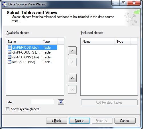
Select all relevant objects (in our case: dimREGIONS, dimPERIODS, dimPRODUCTS, and factSALES).
Next, provide a name for your "Datasource View", like "Test" and click "finish".
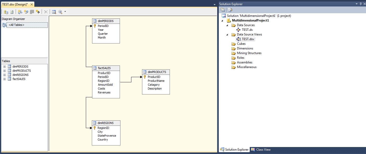
Your Visual Studio screen will alter into a screen similar to figure 7.
Note:
Note that your "Datasource" has the ".ds" extension (in my case "TEST.ds") and the "Datasource View" uses
the ".dsv" extension (in my case "TEST.dsv").
If you browse through the "c:\dwh" folder, you will also see the associated physical files.
Fig 7.
Step 4: Creating the Cube:
Allright, we are all set to create the cube. We have a Datasource to locate the Server and database. And we have a Datasource View
which points to the objects (tables) which form the basis for our cube.
In the Solution Explorer, rightclick the Cubes container, and select "New Cube".
The "New Cube Wizard" will start, which will guide you through the design process.
The "New Cube Wizard" will first present you the "Select Creation Method" dialogbox, where you can choose from
a number of options, like "Create an empty cube", or "Use existing tables".
We already have tables which form the basis for our cube, so please select the "Use existing tables" option.
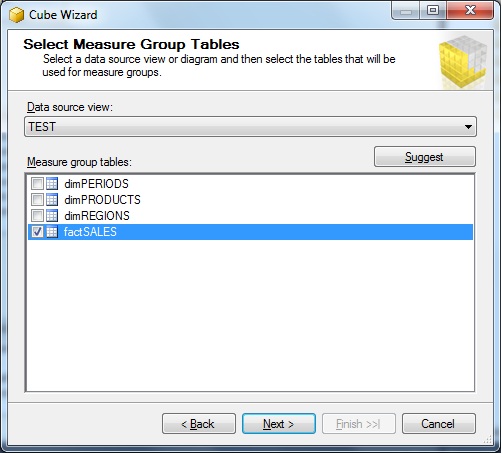
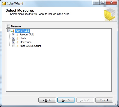
Next, the "Select Measure Group Tables" dialogbox pops up. You know what "measures" are (see Chapter one), so what
is actually meant, is that you select the "fact table" here. So, here we select the "factSALES" object.
Fig 8.
Now the "factSALES tables" indeed contains the "measures", but maybe you want all measures to be in the cube,
or just a selection of certain measures. That's why the next dialogbox enables you to pick all measures, or just a selection.
Here, ofcourse we choose all measures. See figure 9.
Fig 9.
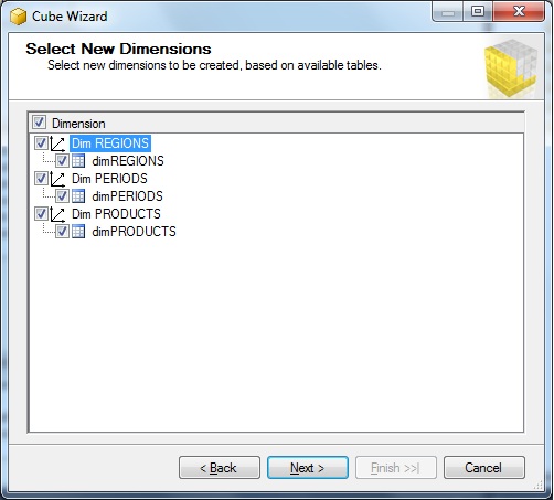
Next, we can choose the dimensions we need in our cube. Here too, we select all our dimensions. See figure 10.
Fig 10.
The last dialogbox, let's you choose a cube name. Here I choose the name "Test", but you can choose whatever you like.
Fig 11.
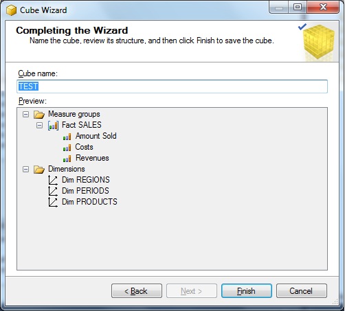
If you click "finish", your are done designing your cube.
Step 5: Deploying the Cube:
Up to now, we have designed the cube, and stored "the source code" in some folder (in my case, it's the folder "c:\dwh").
When you deploy the cube, you register it at the SSAS service. So, the deploying is a neccessary step to take.
First we "build" the cube, hereby creating some binaries, XML files, and a setup script for registering the cube to SSAS.
Then we "deploy" the cube, which actually registers it with SSAS.
From the main menu in Visual Studio, click the "build" option and first choose "Build Solution".
In the output section in Visual Studio, you see output similar to:
------ Build started: Project: MultidimensionalProject1, Configuration: Development ------
Started Building Analysis Services project: Incremental ....
Database [MultidimensionalProject1] : The database has no Time dimension. Consider creating one.
Build complete -- 0 errors, 1 warnings
========== Build: 1 succeeded or up-to-date, 0 failed, 0 skipped ==========
There are 0 errors, but there is 1 warning. The warning is due to the fact that the tables we have used have indeed
no actual field with a Datetime datatype. This is indeed true, so we ignore that warning. Anyway, the build was successfull.
From the main menu in Visual Studio, click the "build" option again, but this time choose "Deploy Solution".
In the output section in Visual Studio, you see output similar to:
------ Deploy started: Project: MultidimensionalProject1, Configuration: Development ------
Performing an incremental deployment of the 'MultidimensionalProject1' database to the 'localhost' server.
Generating deployment script...
Add Database MultidimensionalProject1
Process Database MultidimensionalProject1
Done
Sending deployment script to the server...
Done
Deploy complete -- 0 errors, 0 warnings
========== Build: 1 succeeded or up-to-date, 0 failed, 0 skipped ==========
========== Deploy: 1 succeeded, 0 failed, 0 skipped ==========
Yes, de deployment was successfull!
To actual "fill" the cube with aggregates and data, we need to "process" or "populate" te cube.
Ïn Visual Studio, you richtclick your cube and choose "Process".
However, if it is anticipated that the data volume is very large, this could take some time, and diskspace.
It's quite a seperate science on how you best handle and tune large cubes. Many optimization tips are available,
and if you (are going to) work with large cubes, you still have a lot of research to do.
One thing is already clear: the better optimized the underlying fact and dim tables are, the better performance will be.
Other ways to deploy a cube:
From the Windows Start Menu, you might take a look at the items found under the "Microsoft SQL Server 20xx" -> "Analysis Server".
Here, the Deployment Wizard" can be found.
You can run the Wizard interactively (in a graphical way), or you can use it from the command line.
You might want to investigate what the Wizard can offer you.
Note:
It must further be clear that this simple note does not say anything sensible about tuning cubes.
Indeed, this note is no more than a general and simple overview.
Once "populating" or "processing" has completed, you might view your cube data using Excel 2010, or you might try some MDX queries.
Well.., that's it !