In the series: Note 19.1.
Subject: Quick intro exponential relationship.
Date : 20 October, 2020Version: 0.1
By: Albert van der Sel
Doc. Number: Note 19.1: supplement to note 19..
For who: for beginners.
Remark: Please refresh the page to see any updates.
Status: Ready
Note 19 deals on exponential and logarithmic functions.
This note is a supplement to Note 19, and is a very quick intro
on exponential relationships.
-For more detailed information, it's best to refer to note 19.
-If you only need a very quick intro on the exponential relationship,
then this short note might be useful.
So, this is a stripped version of note 19, with a special focus on "the exponential relationship".
1. Quick intro y=ax and N=gt
An impression of the Analytic description:
In Calculus/Analysis, exponential relations are often described by:y=ax (equation 1)
where a is some constant (like 2, 3, ¼ etc...). In the figure below, you seethe graphs of y=3x and y=⅓x.
The first one, is a steeply rising function, while the second one is a function which
rather quickly decends.
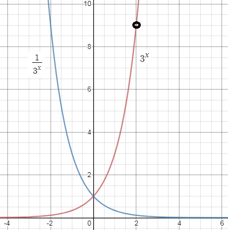
-If you consider y=f(x)=3x, and try some x values like x=-1, x=1, x=2,
then you would indeed agree on the "shape" of that function.
Indeed: f(-1) = 3-1 = ⅓, f(1)=31=3, f(2)=32=9 etc..
-If you consider y=⅓x, and try some x values like x=-1, x=1, x=2,
then you would indeed agree on the "shape" of that function.
Indeed: f(-1) = ⅓-1 = 3, f(1)=⅓1=⅓, f(2)=(⅓)2=⅓ * ⅓ = 1/9 etc..
Ofcourse, you may also see a function like y= c * ax, where "c" is another constant,
which might be larger or smaller than "1". Ofcourse, when c=1, we simply have y= ax again.
In the relation y=ax we must note that:
-If a < 1, the we have graphs like the y=⅓x example
as shown in the figre above. If "x"inceases, then the function decreases.
-If a > 1, we have graphs similar in shape as y=3x as shown in the figure above.
If "x"inceases, then the function increases as well, and the more steeply, the higher "a" is.
An impression of the notation in many practical applications.
In all sorts of studies in biology, sociology, physics, geology etc.., a slightly different notationis used, but that one is completely equivalent to what we have seen above.
Since many researchers, study "something" which varies with "time", the "x" is often replaced by "t" (time).
Also, many studies relate a "number" or "amount" (like the amount or growth of bacteria) with time,
the usual x/y relationship is written as N/t relationship.
So, instead of:
y=ax
we now usually have a notation like:N= b gt (equation 2)
where:-"b" is initial (starting) amount at t=0.
-"t" is time, similar to "x" in the convential notation.
-"N" is the new amount after "t" has passed, in which "b" has growthed (or declined) to "N".
-"g" is the base number, or also called the "growthfactor".
Instead of the usual XY coordinate system, with x and y values, we now have a relation
with N and t values, like if the x-axis is replaced by a t-axis. But fundamentally, nothing hs changed
at all.
where N (or N(t)) is the amount at a certain time (which varies with time), "b" is some initial number
at the starttime t=0, and "t" is time (similar as the role of "x" in the analytic description).
equation 2, works with any suitable unit of time. You might think that t in seconds might be
the preferred choice, but it simply depends on the subject under study.
Sometimes, it's more obvious to use days (like growth of the number of bacteria), and sometimes
it's more suitable to use years (like the acceptance of some social media among users).
Suppose we start with 104 bacteria at day "0".
Every day we measure the number of bacteria. Suppose that "g", the growthfactor, is 1.5.
Then we have:
at day 0: the starting "time": 104
at day 1: 104 * 1.51 = 1.5 * 104
at day 2: 104 * 1.52 = 2.25 * 104
at day 3: 104 * 1.53 = 3.38 * 104
etc..
Although N does not increase extremely fast, it's still an exponential relation, since
we have a constant factor increase per day.
It's quite similar to the behavior of y=3x, where "x" is counted in days.
On day three we would have y=33=27.
On day four we would have y=33 * 3 =34=81.
For every day "difference", we have constant factor of "3".
Let's consider an example of this way of doing business:
Example 1 (with g > 1):
Suppose that you have collected the number of internet users, of a certain city, from the year 2000, up to 2004.Suppose You have found the following data:
| N | Year |
| 30 | 2000 |
| 240 | 2001 |
| 1920 | 2002 |
| 15360 | 2003 |
| 122880 | 2004 |
So, what to make of this data? If the Number at each year, divided by the former number of the
year before that, produces a constant factor, then we are likely to have found
and exponential relation.
Let's try:
122880/15360=8, 15360/1920=8, 1920/240=8 etc..
It seems that we have found, per year, we have a constant factor of "8".
You may say that we have found a "growthfactor" of "8". Each year, the former N
has been multiplied with "8".
Looks like 8t, doesn't it?
Please notice, that this factor works for each year, that is, for each unit of time,
so it's not a linear relation.
If you would look at two years, like this example, 122880/1920= 64 = 82.
You can also try something like that over 3 years, which gives us 83.
The relation thus, smells like something which has a factor like 8t
Also note that we started in the year 2000, up to 2004, meaning that we have 4 timesteps,
namely 2000->2001, 2001->2002, 2002->2003, 2003->2004.
Let's assume that our relation is:
N = 30 8t (with "t" in years)
We take as an initial value, the value of "30", since from that moment on,we have started the measurements.
Would it work?. Let's find out. Using the formula, then over 4 years, the initial value "30"
must have grown to:
N = 30 * 84 = 30 * 4096 = 122880
Indeed, this matches the data of the table above.
Example 2 (with 0 < g < 1):
Suppose we have 1 kg (1000 g) of a certain radioactive substance.This stuff decays into other producs, and suppose we have some sort of technique
to measure the remaining amount of that radioactive substance, over "t".
Suppose further that we have found the following measurements:
| Amount | At time: |
| 1000g | t=0h |
| 700g | t=1h |
| 490g | t=2h |
| 343g | t=3h |
| 240g | t=4h |
Let's see how the amount have changed per hour:
240/343=0.7, 343/490=0.7 etc.. Here, I used the data over 3 hours.
It seems that our relation is:
N = 1000 * 0.7t (with "t" in hours)
Let's do quick check. What would be the remaining amount after 4 hours?N = 1000 * 0.74 = 240g.
That's in accordance with our measurements (see table), so our formula N = 1000 * 0.7t is correct.
2. Half-life and doubling time.
Half-life:Suppose we have found an relation for some amount of "stuff", let's call that amount "N(t)",
which obeys the following relation:
N(t) = b * 0.95t
where b is the initial value at some starting time, then the amount N(t) will decrease as time progresses.
We know exactly how much of the original stuff remains, since we have the expression to calculate it.
Practical applications are for example the halflife time for some radioactive substance.
Suppose that for some radioactive substance, the halflife τ is known. Then after τ time,
half of that radiactive material has decayed.
In the example N(t) = b * 0.95t sketched above, we should have:
½b = b * 0.95t => ½= 0.95t.
(the ½ b is due to the fact that only half of the original amount remains).
So, in this case we must solve for "t" using 0.95t = ½ or, 0.95t = 0,5.
In general:
gt = ½
Usually, you calculate this by using your graphical calculator (or computer).But if you would happen to know logarithmic functions, you would know that, for the example we used above:
0.95t = ½ => 0.95log(½) = t.
So, this might help in finding concrete answers. If you are not so comfortable with logarithms, please see note 19.
Doubling time:
This time, we might have a relation like for example N(t) = b * 1.3t, so that indeed the
growthfactor "g" > 1.
The Doubling time, is exactly that timespan, where the initial value "b" grows to 2b, so:
2b = b * 1.3t => 2 = 1.3t.
So in this example, you must solve "t" from: 1.3t = 2.
In general:
gt = 2
Again, you can rewrite that in a logarithmic form, which might help to solve for "t".But on most Highschools, it's common to use a graphical calculator if "g" is known,
so that you need to solve an equation like 1.3t = 2.
3. Percentages to growthfactor.
Going from a percentage to growthfactor:If something growths or declines with a certain percentage per unit of time, then you can
express that as a growthfactor as well.
-Increase:
If some initial value increases with, say, with 17% per unit of time, then the associated growthfactor is:
g = (1 + p/100) where p is the percentage like 17%
So in the example of 17% increase, we would have g = (1 + 17/100) = 1.17.So, we started out with 100% of the amount, and that grows with 17% per unit of time.
Thus, after the first time unit, we have 117% of the original amount.
This is equal to: b(at t=1) = b(at t=0) * 1.171 = 1.17 b.
This corresponds to 117% b.
Thus the general formula above, seems correct.
-Decrease:
If some initial value decreases with, say, with -17% per unit of time, then we can apply
the same formula, but this time we take into account the negative sign of that percentage.
So in the example of 17% decrease, we would have g = (1 - 17/100) = 0.83.
In the last example, your exponential formula would be: N=N0 0.83t
Note that sometimes I use "b" to denote te initial value (at t=0), and sometimes N=N0 or N=Nt=0.
In case the initial value at t=0 would be, for example "1000", we would have N=1000 * 0.83t
Thus, as usual, you can calculate the current number if you know the number of timeunits "t".
Going from a growthfactor to a percentage:
Without any proof, we state that: