In the series: Note 7.
Subject: The bx, ex, and ln(x) functions.
Date : 4 March, 2016Version: 0.3
By: Albert van der Sel
Doc. Number: Note 7.
For who: for beginners.
Remark: Please refresh the page to see any updates.
Status: Ready.
This note is especially for beginners.
Maybe you need to pick up "some" basic "mathematics" rather quickly.
So really..., my emphasis is on "rather quickly".
So, I am really not sure of it, but I hope that this note can be of use.
Ofcourse, I hope you like my "style" and try the note anyway.
This note: Note 7: The bx, ex. and ln(x) functions.
Each note in this series, is build "on top" of the preceding ones.
Please be sure that you are on a "level" at least equivalent to the contents up to, and including, note 6.
1. Introduction of the "bx" and "ex" functions.
1.1 A few remarks on general exponential functions in the form f(x)=bx.
We by now have seen quite a few types of functions, like linear-, and quadratic functions, polynomials of higer degree,the sin(x) and cos(x) functions etc..
Here we will meet a new class of functions, namely:
f(x)=bx (equation 1)
where "b" is some constant number (like '2', or '5', or '1/2' etc..). The number "b" is also often calledthe "base" number. It's also often called the "growthfactor".
You might generalize the equation a bit, if you like. A description like:
f(x)= a bg(x) like for example f(x)=5 3(x+2) would be in a slightly more general format.
So, a more general format is:
f(x)= a bg(x) (equation 2)
Where a is some number, and "b" is the base, or growthfactor.Note:
In a section below, we will see a notation like N(t) = N0 gt.
Such notation is quite common in all sorts of sciences. You might plot such function in an "N" and "t"
axis system (instead of the usual XY coordinate system).
Ofcourse, nothing fundamental changes if using (N,t), instead of the usual (x,y) system.
These functions are relatively easy to plot. In figure 1 below, I have plotted 6 simple examples, namely:
f(x)=2x, and
f(x)=5x, and
f(x)=0.3x, and
f(x)=2x+3, and
f(x)=-2x, and
f(x)=2(x+2), and
Figure 1. f(x)=2x, f(x)=5x, f(x)=0.3x, f(x)=2x +3, f(x)=-2x, f(x)=2(x+2)
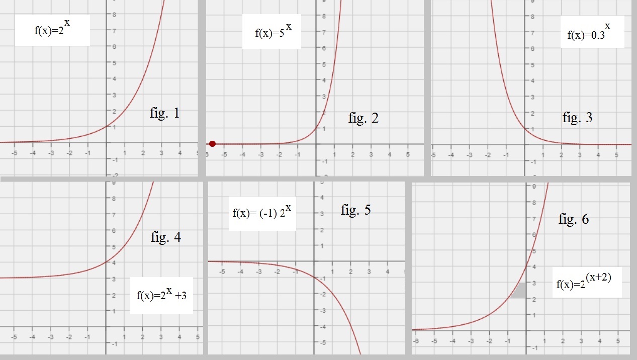
Le's concentrate for a moment on f(x)=2x and f(x)=5x. It's easy to plot them, since having
just a few points, already gives a reasonable picture on how the function "looks like".
Let's first take a look at f(x)=2x
| value of x: | value of y=f(x) |
| x= -2 | y= 1/4, since 2-2=1/4 |
| x= -1 | y= 1/2, since 2-1=1/2 |
| x= 0 | y= 1, since 20=1 |
| x= 1 | y= 2, since 21=2 |
| x= 2 | y= 4, since 22=4 |
| x= 3 | y= 8, since 23=8 |
| x= 4 | y= 16, since 24=16 |
In this case, since we have 2x, the next f(x) is 2 times the former f(x) value.
However, would we have created a table for 3x, the next f(x) would be 3 times the former f(x) value.
Also, would we have created a table for 7x, the next f(x) would be 7 times the former f(x) value.
You can conclude that the larger the "b" (in "bx") is, the steeper the function increases along the +x axis.
Question:
Can you make a similar table for f(x)=5x ?
Here are a few observations:
About the "growthfactor" (base number)
b > 1If b > 1, then a fuction as f(x)=bx has a shape as we have seen above. However, the larger b is,
the faster the function "climbs". Suppose b=10, then when x=3, then f(x)=103 = 1000,
and when x=6, then f(x)=106 = 1000000.
In figure 1, you can clearly see that f(x)=5x, rises much "faster" compared to e.g. f(x)=2x.
All exponential functions bx with b > 1, are rising functions.
0 < b < 1
If 0 < b < 1, then a function as f(x)=bx has a shape similar to subfigure 3, in figure 1.
These functions decline fast. For example, for f(x)=0.3x it is true that if x=2, then f(x)=0.32 = 0.3 x 0.3 = 0.09,
and if x=3, then f(x)=0.33 = 0.3 x 0.3 x 0.3 = 0.027.
All exponential functions bx with 0 < b < 1, are declining functions.
About the Asymptotes
Note that those functions exhibit asymptotic behaviour.-For example, if we look at f(x)=2x, and f(x)=5x, then if we move to the -x direction,
the graphs go nearer and nearer to the line "y=0", but it will never exactly reach "y=0".
-However, if we "lift" such a function upwards, by adding a constant like with f(x)=2x+3,
(see subfigure 4 in figure 1 above) then the asymptote has shifted too. In this case, the asymptote now
is the line "y=3".
-Thus note that a function f(x)=bx, with some constant added, like f(x)=bx + 3, or f(x)=bx -2,
can be regarded as a simple shift, upwards, or downwards, along the y-axis. It's a translation
Up or Down, of the entire graphic. Thus the Asymptote shifts too (compared to bx).
1.2 The exponential function f(x)=bx when "b"=e.
The number "e" is approximately 2.7. It's a real number (element of ℝ), but cannot be written as a fraction.As with any exponential function bx (with b>1), it's a rising function, in the positive x direction.
In this case, the function must be written as:
f(x)=ex (equation 3)
As as graph, f(x)=ex is vey similar to the graphs we have seen above (where b > 1).So, you might say that we have not much "news" here.
But "e" truly is a special number, as is discussed in the next section.
Figure 2. f(x)=ex
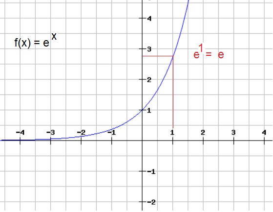
Ofcourse, when x=1, we have f(x) = e1 = e.
Note in figure 2, that e is about 2.7.
1.3 Some background on "e".
Around the year 1683, Jacob Bernoulli found that as "n" goes to infinity in the following expression,
the outcome "converges" to a very specific number. Today we call that specific number 'e'.
lim n → ∞ (1 + 1/n)n = e.
So, if you would say: let's take n=100, then the expression would be (1 + 1/100)100Let's do some calculations. If you would calculate (1 + 1/10)10 then we have 2.59.
if you would calculate (1 + 1/100)100 then we have 2.70.
You see, if we only take n=100, then we are already pretty close to the "true" 'e'.
You get more and more closer, the larger 'n' is.
People with a background in economics or accounting would see a rather familiar formula.
It resembles the formula when you set away an amount of money, to a certain rate of interest, for period of "t" (n).
The formula "(1 + 1/n)n" seems to be fundamental to describe a sort of accumulated growth with a constant interest rate.
Yes, but what about physics? Just too much examples are available. Here is one that that also resembles the above.
Suppose you have N0 particles of radioactive material. Each nucleus has a certain "chance" to decay. But as a statistical ensemble,
which is a very high number of such nuclei, each have a (general) expectation value to decay.
Say that this expectation value is 6 hours, and you single out one of such nuclei, then there still is a chance
that you stare to it for several years. But on average, each nuclei has a good chance to decay in about 6h.
The "half-life" is defined to be that time, that halve of the material has decayed (with a very high probability).
The amount of original (not decayed) nuclei, can be described by:
N(t)= N 0 e -kt
In this case the e -kt factor, resembles the utmost right curve in figure 1 a bit, as of x > 0.
Many natural processes can be described using expressions, where 'e' plays a major role, especially at
all sorts of events where an "ensemble" growths or declines.
What is that with "e"? I don't think it's only math or physics. I bet that it's a matter for philosophy too.
2. Common Usage of exponential functions in real research.
2.1 Introduction.
In many researches in physics, biology, or social researches, folks study a process which is evolving over time.For example, a certain initial amount of bacteria, under favourable circumstances for those living creatures,
start to grow according to an exponential relation. So, the number increases and that number is often denoted by "N".
However, instead of the usual x-axis and y-axis, the researchers plot the relation as N related to time (t).
Ofcourse, there is no fundamental difference in taking an N-axis and t-axis. It's exactly the same as
in using a x-axis and y-axis.
In many comparable studies as was sketched above, the relation used, is expressed as:
N = b gt (equation 4)
or, sometimes written as (or similar):N(t) = N0 gt (equation 5)
In this formula, we have:-"b" is initial (starting) amount at t=0. Similar for N0 in equation 5.
-"N" is the new amount after "t" has passed, in which "b" has growthed (or declined) to "N".
-"g" is the base number, or also called the "growthfactor".
There is really no fundamental difference when you compare equation 4, to for example f(x)=2x.
Ocourse, instead of "x", we now consider the time "t" as the variable, which is plotted horizontally,
just fully similar as to the x-axis.
Furher, we have the exact same behaviour with "g", as we already have seen in chapter 1.
That is:
For g > 1: we have a rising function (comparable to e.g. 2x).
For 0 < g < 1: we have a declining function (comparable to e.g. 0.3x).
Most often, "g" is also called the "growth factor".
However, in many cases there will indeed be growth (g > 1), but in many other cases, an initial amount
will decline over t, just like for example "0.3x" is a declining function as x increases.
-Thus, if you see the relation N = b gt and g is "> 1", then you will immediately know
that the initial amount will increase over time.
-Thus, if you see the relation N = b gt and it is true that "0 < g < 1", then you will immediately know
that the initial amount will decrease over time.
Also note that the starting value, "b", is the amount at "t=0" (or some moment defined as t=0).
You can easily check that with:
N = b gt => for t=0 => N = b g0 => N = b * 1 = b (at t=0).
2.2 Examples: Interpreting table data, and see if an exponential relation exist.
How "t" is measured, depends completely on the specific situation and the system you are studying.The time "t" could have been measured in seconds, or months, or years...
In Physics, many physical processes are measured in seconds, or fractions thereof.
In Biology, for example the study of the growth of bacteria, might be sampled in hours, or days.
Let's take a look at a few examples.
Example 1 (with g > 1):
Suppose that you have collected the number of internet users, of a certain city, from the year 2000, up to 2004.
Suppose You have found the following data:
| N | Year |
| 30 | 2000 |
| 240 | 2001 |
| 1920 | 2002 |
| 15360 | 2003 |
| 122880 | 2004 |
So, what to make of this data? If the Number at each year, divided by the former number of the
year before that, produces a constant factor, then we are likely to have found
and exponential relation.
Let's try:
122880/15360=8, 15360/1920=8, 1920/240=8 etc..
It seems that we have found, per year, we have a constant factor of "8".
You may say that we have found a "growthfactor" of "8". Each year, the former N
has been multiplied with "8".
Please notice, that this factor works for each year, that is, for each unit of time,
so it's not a linear relation.
If you would look at two years, like this example, 122880/1920= 64 = 82.
You can also try something like that over 3 years, which gives us 83.
The relation thus, smells like something which has a factor like 8t
Also note that we started in the year 2000, up to 2004, meaning that we have 4 timesteps,
namely 2000->2001, 2001->2002, 2002->2003, 2003->2004.
Let's assume that our relation is:
N = 30 8t (with "t" in years)
We take as an initial value, the value of "30", since from that moment on,we have started the measurements.
Would it work?. Let's find out. Using the formula, then over 4 years, the initial value "30"
must have grown to:
N = 30 * 84 = 30 * 4096 = 122880
Indeed, this matches the data of the table above.
Example 2 (with 0 < g < 1):
Suppose we have 1 kg (1000 g) of a certain radioactive substance.
This stuff decays into other producs, and suppose we have some sort of technique
to measure the remaining amount of that radioactive substance, over "t".
Suppose further that we have found the following measurements:
| Amount | At time: |
| 1000g | t=0h |
| 700g | t=1h |
| 490g | t=2h |
| 343g | t=3h |
| 240g | t=4h |
Let's see how the amount have changed per hour:
240/343=0.7, 343/490=0.7 etc.. Here, I used the data over 3 hours.
It seems that our relation is:
N = 1000 * 0.7t (with "t" in hours)
Let's do quick check. What would be the remaining amount after 4 hours?N = 1000 * 0.74 = 240g.
Example 3: The growthfactor over other "timeunits".
In example 1, we found a growthfactor of "8".
For convience, the data of example 1 is repeated here:
| N | Year |
| 30 | 2000 |
| 240 | 2001 |
| 1920 | 2002 |
| 15360 | 2003 |
| 122880 | 2004 |
Our methodology was to take the value of Ni and devide that by the directly former
value of Ni-1, for example, "122880/15360 = 8".
And we repeated that procedure for other consecutive years.
But what if, you want to evaluate the growthfactor over e.g. 2 years, instead of one?
In this example, the growthfactor will be 8x8 = 82 = 64. You can also calculate it
by using the N values of those "n" years, like for example "122880/1920 = 64 = 82".
So, for the growthfactor, over "n" timeunits, that factor will be gn.
Change of the unit of time.
-If you have a data table, and you go for example from a unit of one year to a unit of "n" years,
then your growthfactor changes to:
g → gn
This is true not only for years, but works the same for going from months to years,
or from units of 10 sec to units of 100 sec etc..
-If you have a data table, and you go for example from a unit of time, to "n" smaller units,
then your growthfactor changes to:
g → g1/n
This is true not only for years going to months, but works the same for going from months to weeks,
or from units of 100 sec to units of 10 sec etc..
2.3 Going from a percentage to growthfactor, and the other way around.
Going from a percentage to growthfactor:If something growths or declines with a certain percentage per unit of time, then you can
express that as a growthfactor as well.
If some initial value increases with, say, with 17% per unit of time, then the associated growthfactor is:
g = (1 + p/100) where p is the percentage like 17%
So in the example of 17% increase, we would have g = (1 + 17/100) = 1.17.In this example, your exponential formula would be: N=N0 1.17t
In case the initial value at t=0 would be, for example "1000", we would have N=1000 * 1.17t
If some initial value decreases with, say, with -17% per unit of time, then we can apply
the same formula, but this time we take into account the negative sign of that percentage.
So in the example of 17% decrease, we would have g = (1 - 17/100) = 0.83.
In the last example, your exponential formula would be: N=N0 0.83t
In case the initial value at t=0 would be, for example "1000", we would have N=1000 * 0.83t
Going from a growthfactor to a percentage:
Without any proof, we state that:
p = (g - 1) * 100 where p is the percentage, g is the growthfactor
Next, let's discuss the ln(x) function.3. Introduction "ln(x)".
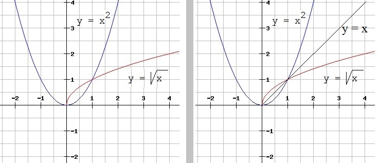
3.1 Inverse function in general.
Suppose you have the functions u and v, in such a way, that u(v(x))... is x again !Well, it's not uncommon to have such functions. Suppose we have these two:
u(x)=√ x
v(x)=x2
Then u(v(x))= √ (x2) = x.
So, if we let "v" operate on x first, en then let "u" operate in "v(x)", we have x again. So, if both functions
are applied, then nothing happens to "x". The funcion "u(v(x)" maps "x" onto itself.
If we look at these two again:
u(x)=√ x
v(x)=x2
Then people also often say, that "v" is the inverse function of "u", and the other way around.
When two functions are related in such a way, people often do not talk of 'u" and "v" functions,
but the use the f anf f-1 notation.
Thus: f(f-1(x)) = f-1(f(x)) = x
The functions "f" and " f-1" are both each others inverse function.
Note: (optional reading)
In other mathematical disciplines, like that of studying vectors, matrices etc.., when a "mapping" or "operator" A
has an inverse operator, A-1, then it is often said that "A A-1 = I",
where I is the Identity operator, or "the doing nothing" operator, which nicely sums it up.
Let's plot both √ x and it's inverse x2 in the XY plane.
See figure 3. Note that if you would also plot the line "y=x", then it becomes visible that both functions
are "mirrored" through "y=x".
Ofcourse, when we say "x is mapped onto itself", it means the line y=x, since that function is f(x)=x,
thus for example f(f-1(x))=x, means that f(f-1(x)) really is the same as y=x.
Figure 3. x2 (in blue) and √x (in red) x
3.2 ln(x) as the inverse function of ex.
Another class of functions are the logarithmic functions. In many technical applications and stdies,the logarithmic function using the number '10' as it's "base", is very helpful.
A couple of examples may illustrate that.
The "claim" here, is that if g(x)=ex, then it's inverse function is h(x)=ln(x).
But, if that is true, then h(x)=ln(x), must be the inverse function of g(x)=ex.
We know how the the curve of ex looks like. Then, the inverse function must be the mirror with respect to f(x)=x.
Indeed, ofcourse it's possible to draw such an inverse curve, since you only need to mirror ex in f(x)=x.
Sure, it would be great to prove it. However, I can't prove it right now, since I like to do that using a primitive function.
Figure 4. g(x)=ex and h(x)=ln(x)
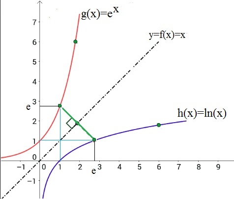
Thus, if they are each others inverse, then it should be true that:
ln(ex) = e ln(x) = x
3.3 The derivatives of ln(x) and ex.
Ofcourse we need to know the derivatives of both functions.1. The derivative of ex:
From note 5, we know that the fundamental relation for "the rate of change" is:| lim h -> 0 | f(x + h) - f(x) ---------------- h |
It's important to know, that the upper equation really is the "heart" of finding derivatives.
If needed, please check note 5 again, where the relation is fully explainend.
Now, using "ex" in the equation:
| lim h -> 0 | e(x + h) - ex ---------------- h |
Remember from note 1, that an+m = an am, where a can be any number.
Thus:
| lim h -> 0 | ex eh - ex ---------------- h |
Now, we can "factor out" ex:
| lim h -> 0 | ex (eh - 1) ---------------- h |
So, we may write that as:
| ex lim h -> 0 | (eh - 1) ------------ h |
Note: Do you see that we have managed to pull out ex from the Limit?
While the Limit itself converges to "1" (I should have proved that too), we have found the very remarkable fact, that:
If f(x)= ex then
f '(x)= ex
or:| d ex ------ dx |
= ex |
This fact, that the derivative of a function is itself, has amazed countless mathematicians and philosophers.
Indeed. It's a very remarkable fact. But we also know that ex is involved in accumulated natural growths
So, it might be argued, that it's very remarkable status, should not surprise us at all.
2. The derivative of ln(x):
Here we do not provide for a proof. I'am afraid to "clutter up" my notes too much, while they are intendedfor "quick" introductions in math. But I really like you to remember the following:
If f(x)= ln(x) then
f '(x)= 1/x
(for x>0)
or:
| d ln(x) ------ dx |
= 1/x |
Note that the function 1/x, shows asymptotic behaviour if "x" approaches "0".
We have seen 1/x before, so we were already aware of that fact.