Chapter 1. What is a Fourier expansion (or Fourier series)?
Let y=g(x) represent any (continuous) periodic function. Then it can be represented by a seriesof sin(Nx) and cos(Nx) functions (where N are integer numbers, so that for example a member in the series is "sin(5x)").
Note the fact that the sin(Nx) and cos(Nx) resemble "basis" vectors. Indeed, in note 12 you saw that a vector can
be written as a superposition (or a sum) of unit- or basis vectors.
Here is Fourier's basic expansion:
g(x) = a0 /2 + Σ n=1∞ ( an cos(nx) + bn sin(nx) )
= a0 /2 + a1 cos(x) + b1 sin(x) + a2 cos(2x) + b2 sin(2x) + a3 cos(3x) + b3 sin(3x) + ...
Please note that the "n"'s are simply integers, so n=1, 2, 3, 4, ......Also, generic formula's are provided by the theory, to find the coefficents like a1, b1, a2, b2 ... etc..
Although the series is "infinite", it's truly amazing how close you can resemble any function g(x), by taking
for example, as low as only 7 pairs of sin() and cos() terms.
The more terms you add in the sum, the more precise you get.
The "x" interval where the function g(x) is equated to the expansion (the sum in equation 1), is often at first limited
to the period T of g(x) (like for example the interval [0-π], or [-π-π] etc..), or whatever the period is.
This is done to to calculate the coefficients like "bn".
Below is an example that will hopefully make it "likely" (or convincing), that such an expansion is really possible.
1.1 How to make it plausible.
Example 1:Suppose you would start with a function which does not resemble a sin() or cos() at all.
We could take one of the "famous" examples, like for example a sawtooth graph, or a square wave graph.
Let's investigate a square wave. In figure 1 below, in the upper left corner we see a square wave.
Figure 1. Representing a "square wave" by a small number of sinus harmonics.
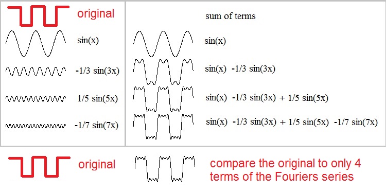
Although it's not proven right now, but if we just take a few terms of a Fourier expansion:
sin(x)
-1/3 sin(3x)
1/5 sin(5x)
-1/7 sin(7x)
and we simple add those terms, then we get g(x) = sin(x) - 1/3 sin(3x) + 1/5 sin(5x) - 1/7 sin(7x)
In the lower right, you can see the graph of this superpostion. It's remarkable how much the result
already resembles the original square wave.
You can probably imagine, that if we would take, for example, 50 terms of the expansion,
then the resemblence would be very precise.
1.2 Fourier series or Fourier expansion.
As already listed above, a Fourier expansion of a periodic function is:g(x) = a0 /2 + Σ n=1∞ ( an cos(nx) + bn sin(nx) )
= a0 /2 + a1 cos(x) + b1 sin(x) + a2 cos(2x) + b2 sin(2x) + a3 cos(3x) + b3 sin(3x) + ... (equation 1)
Most often, the analysis of functions g(x) is done over the "Period" of g(x), like for example the interval on the x-axis,where x in [0, π], or [0, 2π], or [-π π].
Suppose the Period of g(x) is the interval [-π, π]. So, the period of g(x) is 2π
The coefficients an and bn, are calculated as follows:
an = 1/π ∫-π π g(x) cos(nx) dx (equation 2)
bn = 1/π ∫-π π g(x) sin(nx) dx (equation 3)
a0 = 1/π ∫-π π g(x) dx (equation 4)
So, why does these coefficents (as of a1) must be calculated that way?Let's take a look at, for example, b3. This the coefficient for sin(3x).
In general, suppose that b3 would be large, then the contribution of sin(3x) to the series would be large.
In general, suppose that b3 would be very small, then the contribution of sin(3x) to the series would be very small.
Thus the coefficient, like b3, determines how much the component (like sin(3x)) contributes to the series.
Many interpret it this way: The integral of "g(x) sin(3x)" over the interval [-π, π] is equivalent
to the average (or "weighted") contribution of sin(3x) to the expansion.
However, it's true that as "n" increases, the associated terms quickly get's smaller and smaller.
Note:
The coefficient (or number actually) "a0", which is the first term in the series, has a rather special status.
You may interpret it as the average value of g(x) over the "period" (like the interval [-π, π]).
Maybe you still have problems in understanding the coefficients like an.
As said above, you may interpret them als the "weighted average" contribution of sin(nx) or cos(nx)
to the expansion.
However, you may also view equation 1 in the sense of a vector expansion of g(x) on the basis vectors "sin(nx)" and "cos(nx)".
In that sense, you can view the coefficients in the same way as you would view the vector components, written out
as the sum of unit-vectors.
So, it looks like an expansion of vector A on unit vectors. For example, if A=(7,18,1) then A= 7 (1,0,0) + 18 (0,1,0) + 1 (0,0,1).
The contribution of (0,0,1) to A is rather small. As you know from note 12, for example "7", is the projection of A on (1,0,0).
Thus:
an = 1/π ∫-π π g(x) cos(nx) dx
then "resembles" the component of g(x) on cos(nx).Thus, g(x) in equation 1, is formed from a (infinite) superpostion of basis vectors, and the coefficients
can be interpreted exactly like you did in vector calculus.
The whole purpose of Chapter 1, was to give you a "reasonable" impression on how a Fourier expansion works.
If that worked, then for now, it's good enough for me.
Chapter 2. Taylor series.
This subject resembles a bit, what we have seen in Chapter 1, in the sense that a function can be expanded in mathematical terms.While Fourier developed this insights of the expansion of a function around 1800, Taylor developed his own type
of expansion around 1714. But it was not before Lagrange in 1772 re-discovered it's power, that Taylor's work became
really famous. No doubt the work inspired many ohers and pushed differential calculus forwards.
All in all, it's a different approach from the Fourier series. Here is the general equation of a Taylor series:
| f(x) = | f(a) + |
f '(a) ---- 1! |
(x-a) + |
f ''(a) ---- 2! |
(x-a)2 + |
f '''(a) ---- 3! |
(x-a)3 + | ... (equation 5) |
Ofcourse, we reckognize the first derivative f'(a), the second derivative f''(a) etc..., all calculated in x=a.
Yes, that's really remarkable. Just choose a point x=a on the x-axis. Then calculate the derivatives f', f'', f''' etc..
and multiply each derivative with a corrseponding power of "(x-a)", just like you can see in equation 5.
It turns out that you then can "calculate" f(x), for any x.
Just like with Fourier series, the Taylor series get more precise too, if you add more terms to the series.
The denominators like "2!" and "3!"(or more generally, the "n!") you see in equation 5, is a shorthand notation.
It means this:
1! = 1
2! = 2 x 1
3! = 3 x 2 x 1
4! = 4 x 3 x 2 x 1
etc..
Examples:
Example 1: Taylor Expansion of f(x)=ex:
Let's try to expand ex. It's actualy a simple example, since from from note 7, you might rememberthat the derivate of ex, is ex again! Indeed, it's true for all derivates of ex
If needed, check out note 7 again.
And, we will pick x=0, as the "x=a" in the general equation (equation 5).
So, we have:
| ex = | e0 + |
e0 ---- 1! |
x + |
e0 ---- 2! |
x2 + |
e0 ---- 3! |
x3 + | ..... |
| ex = | 1 + | x + |
x2 ---- + 2! |
x3 ---- 3! |
+ ..... |
Example 2: Taylor Expansion of f(x)=cos(x):
Here we will choose "a=0" too.Remember from note 5, that:
If f(x)=sin(x) then f '(x)=cos(x)
If f(x)=cos(x) then f '(x)= -sin(x)
So, we have:| cos(x) = | cos(0) + |
-sin(0) ------ 1! |
x + |
-cos(0) ------ 2! |
x2 + |
sin(0) ------ 3! |
x3 + |
cos(0) ------ 4! |
x4 | + | ..... |
| cos(x) = | 1 | - |
x2 --- 2! |
+ |
x4 --- 4! |
+ | ..... |