This note is especially for beginners.

Maybe you need to pick up "some" basic "mathematics" rather quickly.
So really..., my emphasis is on "rather quickly".

So, I am not sure of it, but I hope that this note can be of use.
Ofcourse, I hope you like my "style" and try the note anyway.

Chapter 1. The "Population" mean- and Standard deviation.

For the "average" or "mean", and "standard deviation" for grouped data into classes: see Chapter 3.
This chapter, and chapter 2, will discusss the average (mean) and the standard deviation for "un-grouped" data (just a bunch of numbers).

"Un-grouped" data means that we have not placed (or classified) data in "equi spaced intervals" (histogram-like).
In this chapter, and chapter 2, we assume that we have "just" a (small or large) series of data or measurements.

But even here, two "forks" exist:

1. We have access to all data. That is, we analyze the whole population (Chapter 1).

2. We have only a "sample" of "n" items or measurements from a (much) larger "Population of N items" (Chapter 2).

The differences between (1) and (2) are not "shocking". However with (2), we automatically have introduced
somewhat more uncertainty in a key value like "the standard deviation".
But, those differences gets less relevant if the number of measured events in the sample gets larger. That is, if n->N.

This will all be explained in chapters 1 and 2. I promise: Just read both chapters, and it will become clear.

As said before, this chapter deals with statistics over a whole "Population" (access to all data).

1.1 The "average" (or "mean value").

The "average" (or mean value), the "median", and the "standard deviation" are absolutely key values in statistics.
These key values are rather intuitive, and easy to understand.

Suppose you have to determine the average weight of 10 containers.
So, first you weight all containers and write the values in a table.

Here are your results:

container #	weight
container 1	15
container 2	10
container 3	45
container 4	37
container 5	20
container 6	31
container 7	35
container 8	40
container 9	19
container 10	22

To determine the "average" weight, or the "mean" weight, you sum all values, and devide it by 10.
Thus:

mean value =

15+10+45+37+20+31+35+40+19+22 -----------------------------------------------               10

= 23 kg

An average, is a sort of computed "mid point" of a set of values. Indeed: it's an average.

In many textbooks, or articles, the mean is often denoted by the μ symbol.

In general, if you have "N" values a₁, a₂, ..., a_N
And you need to compute the mean value, you would thus calculate:

mean value μ =

a1 + a2 + ...+ aN --------------------------               N

=

1 --- N

Σ ai       (equation 1)

The "Σ" symbol is a shorthand notation for a large summation. So Σ a_i means
that we sum all a_i, where i runs from 1 to N.

Now suppose, that one of the containers was 200kg. That would influence the mean value enormously!

While an average has been the formost measure of a mid-point in a series of samples,
it has the disadvantage of being affected by any single value being much too high or much too low compared
to the rest of the measurements.

That's why in cases, where a few exceptionally high or low values are present, in comparison
to the very large majority of measurements, the median might be more appealing.

1.2. The "median" (as an alternative for the "average or mean"):

This sort of middle value, is not sensitive for an exceptionally high or low value among the samples.

It's simply that value, that "sits" in the middle of all values. So, it sort of seperates
the lower halve, and upper halve, of all values.

Suppose that we have the following measurements:

10,11,14,8,7,16,17,11,20,6,500.

here, the number "500" seems completely "out of line".

However, the average of those values is, computed with our general equation: 620/11 = 56.36.

There might be arguments to discard that "500" (possible measurement error?).
Then we might have a more representative (?) average: 120/10 = 12.

However, if we do not discard any measurement, and order the values from low to high:

6,7,8,10,11,11,14,16,17,20,500.

Then "11" sits in the middle (5 values equal or lower, and 5 values equal or higher, out of 11).

-In case of an uneven set of values, there exists indeed one value which sits exactly "in the middle".
-If there are an even set of values, usually the average if the two centre values are taken.

So, in certain cases, the median might be a more representative value, if you have
no sound arguments to discard exceptionally high or low values.

However, the "mean value" (the average), as computed in equation 1, is generally accepted to be
the most important middle "value" of a full set of measurements.

1.3. The "standard deviation":

Usually, when you have a series of measurements (and associated values), you calculate the "mean" (or "average").
Ofcourse, there are values below- and above the mean.

You can also calculate another sort of average: how far, on “average”, are the data from the mean?

Or, in formal words: "what is the standard deviation from the mean?"

What we learn from that number, is whether most of the data are in a narrow band around the mean,
or in a wider band around the mean.
How "far" a values is from the mean is, is expressed in a "difference". Let's illustrate that with this example:

Example:

Suppose that we have the following measurements:

14,22,14,17,18,24,22,22,23,18,16

Then the mean value is

mean value =

14+22+14+17+18+24+22+22+23+18+16 --------------------------------------------------------                   10

=

160 ---- 10

=16

Then the "standard deviation" σ is calculated as (will be explained):

σ =

√

(

1 --- N

Σ (ai - μ)2

)

=

4.8

Here then, μ=16, N=10, and a_i interates through the list of values.
You can work it out yourself, and using a spreadsheet for example, it's quite easy to do.

Explanation:

The "distance" of a certain value in the series, say "14", to the mean value of "16", is |14-16|= 2.
The "distance" of another value in the series, say "22", to the mean value of "16", is |22-16|= 6.
etc..

So, if we have a listing of values a_i, then we would calculate the difference as |a_i - μ|

Here I use the || symbols, to denote that we only want to know the absolute value, that is,
we only want the value itself, as a positive number, and we are not really interested in the "sign".

Indeed, for example, 22 is "6 steps" from the mean (16), and it's only that difference we are interested in.

Now you could say that we then device an equation like the next one, the determine the "standard deviation":

=

1 --- N

Σ |ai -μ|     (not the generally accepted equation)

Here a_i represents the i^th value, and μ is the mean value.

That would not be unlogical, but it's NOT the universally accepted "average deviation".
However, if you compare it to equation 1 from section 1.1.1, it really looks like an average deviation.

No, it was agreed among mathematicians to use the following measure of the standard deviation:

σ =

√

(

1 --- N

Σ (ai - μ)2

)         (equation 2)

Example illustrating "narrow band" and "wide band":

=>If you would have the values:

10,11,12,8,9,10

Then:

μ = 10
σ = 0.77

Here, σ illustrates that the values are pretty "narrow" around the mean μ
Namely, σ is much smaller than μ.

=>If you would have the values:

10,50,20,120,70,30

Then:

μ = 50
σ = 28

Here, σ illustrates that the values are pretty "wide" around the mean μ
Namely, σ is not much smaller than μ. It's even about the half of the average !

It's thus important to know, that σ "tells" us how "spreaded" the data is compared to the average.
For example, if σ is low (compared to the average), then most data values are "close" to the average.

1.4 Variance.

There is another measure of "the spread" of values around the mean value.
It's called the variance.

In "plain" statistics, it's really no more than the square of the standard deviation.
Or, in orther words, the standard deviation is the square root of the variance.

So, "variance" is no more than the square of the standard deviation, or:

Var= σ²

Often, the variance is denoted by "var" or sometimes also by "s".

Since they are directly related, folks can use "var" and σ interchangably.
If we repeat equation 2 again:

σ =

√

(

1 --- N

Σ (ai - μ)2

)         (equation 2)

Then:

var =

1 --- N

Σ (ai - μ)2        (equation 3)

So, if in examples (like above), you see that the σ was calculated, it's easy to obtain the variance.

In plain statistics, except for the square root, you do not notice any difference.
However, in some advanced topics, it turns out that in some cases they have different interpretations.
For a simple note as this one, it's not an issue at all.

Chapter 2. "Sample" mean and "Sample" Standard deviation.

In chapter 1, we could access all data, often called "Population' statistics".

More often, you are only able to study a "sample" from the the whole population.
If you want to "measure" the opinion of millions of people in a country,
then usually, you are not able to interview all of them. So, you try to get a representative "sample"
from the whole population. Intrinsincally, you introduce some more "uncertainty".

If the number of data elements you measure ("n"), gets larger and larger, then the difference between
"Population" mean and Standard deviation, "Sample" mean and "Sample" Standard deviation,
will more and more narrow down (theoretically).

In population statistics (chapter 1), it is argued that if you can access or "see" all data, that is "N" events or "N" values,
then ofcourse you can calculate the "exact" mean μ and the "exact" standard deviation σ.
It is then rather logical to use "N" as the value of the denominator. You simply have N values.
Here I repeat equations (1) an (2) again:

mean value μ =

a1 + a2 + ...+ aN --------------------------               N

=

1 --- N

Σ ai       (equation 1)

σ =

√

(

1 --- N

Σ (ai - μ)2

)         (equation 2)

Note that "N" is the number of elements in the population.

Also note that μ and σ, are the (more or less) "official" symbols for the population mean
and standard deviation repectively.

In a way, you might say that we are not really doing "statistics" here. Why? We just have "N" values,
and we are, for example, able to calculate μ exactly.

It's in reality more typical that we can only analyze a "sample" from the Population.
Here, a sample consists of a number of observations from the population, but that number is
typically much smaller compared to the population as a whole.

The equations to obtain the socalled "Sample" mean and "Sample" Standard deviation, look very similar,
but for the "sample" Standard deviation, there is a small difference.

So, suppose you have found, or measured, "n" (b_i .. b_n) values (from a much larger Population),
then the "sample" mean value x̄ and the "sample" standard deviation "s", are:

x̄ =

=

1 -- n

Σ bi       (equation 3)

s =

√

(

1 --- n-1

Σ (bi - x̄)2

)         (equation 4)

Why do we devide by "(n-1)" instead of just "n"?

There exists arguments that consider the "degrees of freedom" comparing "population-" and "sample"
deviations. We do not have to make it that complex.
It's actually quite easy:

While we are considering only "n" values from a much larger population, there is a serious risk
of a certain amount of bias.

If we calculate "s" using a division by (n-1), then "s" is larger than just by deviding by "n".
This is exactly what we want. A larger "s" means simply a somewhat larger deviation, which is really true,
since you can only have a smaller deviation by considering the whole population.

So, here we have a "reasonable construct". Deviding by (n-1) increases "s" somewhat (compared by
devision by "n"), thus increasing "s" somewhat, on purpose.

As a simple example, "10/(6-1)" = "10/5" = 2, is larger than "10/6" = (about) 1.66.

Indeed, a larger (or wider) sample standard distribution, designates that we can expect (somewhat) more spreading
around the mean value.

Note that "x̄" (x bar) and "s", are the (more or less) "official" symbols for the "sample" mean
and "sample" standard deviation repectively.

Chapter 3. Average, standard deviation, and Frequency distributions for "grouped data"

In Chapter 1, I often simply used a series of values (a bunch of numbers) in my examples, and illustrated the calculation
of the average, median, or standard deviation.

That's all well ofcourse, but in many cases, the approach is a little different.

Most often "equal spaced" intervals (or "classes") are used, and then we count how many events fall
in each interval.

Key values as average, or standard deviation, then must be obtained using a slightly different approach.

3.1 Histograms, and Distributions.

"Frequency Distributions" are quite simple to illustrate. Let's try ab example.

Example:

Suppose you want to know how many people vote "left", with repect to their age.

Then you could use "equi spaced" intervals, like the age in 20y-24y, age in 25y-29y, age in 30y-34y, etc...
Then, for each such interval, you phone (or try to contact) 100 people, and ask what they are going to vote for.

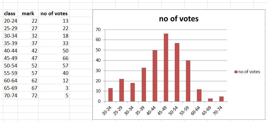
What you might get is something like counting 30 votes in 20y-24y, 60 votes in 25y-29y, .., etc...

You might then create a "Histogram", where on the "x-axis" (horizontal axis), you place your intervals,
and on the "y-axis" (vertical axis), you mark the counts for each interval.

The "equal spaced" intervals, are sometimes also called "classes" or "class intervals".
For example, the class 20y-24y, has two "class limits" (20, 24), and a "class mark", which is the middle number
in that class (22). And it has a "class width" of 5, as all other classes have.

In our example, we might have found the values (counts) for each class, as illustrated in figure 1.
The figure is called a "frequency distribution", and the type of graph choosen here, called is a "histogram".

Figure 1. A frequency distribution, displayed in a "histogram".




You might ask: How would you address the "mean value" and standard deviation in such an frequency distribution?
That would be a very good question. We are going to discuss that in section 2.2.

3.2 The average and standard deviation for "grouped" data, in classes.

In the example above, I used the term "number of votes". But actually, it's the frequency,
or the number of counts, per class.

When calculating something like the mean value, we need to have to take into account the number of counts,
that is, the frequency.

This is a difference with chapter 1.
Essentially, in chapter 1, we had a bunch of numbers, where each of them, had a frequency of "1".

When viewed from that perspective, you might already understand right away, that we now must multiply
each class "midpoint", with the frequency in that class.

Here are the equations for the mean value and standard deviation. I will illustrate thus further in the example below.

Determining the mean value for grouped data in classes:

μ =	Σ fi mi --------      (equation 5) Σ fi

where "Σ f_i" in the denominator, is the sum of all frequencies. This is the "sort of" equivalent
to the "N" of equation 1.

or, as an equivalent equation:

μ =	Σ fi mi -------      (equation 6)  N

Where:

N: is sum of all frequencies (Σ f_i)
m_i: is the midpoint (or class mark) of each class
f_i: stands for the frequency of each class

Determining the Standard Deviation for grouped data in classes:

σ =

√

(

1 --- N

Σ fi (mi - μ)2

)         (equation 7)

Since this all is about a "sample" from a larger "population", you might say that
we have to use "1/N-1" in equation 7 above.
That's right.

But don't forget that statistics over "samples" has an intrinsic uncertainty anyway.
So, in a rather "formal" way: yes, use "1/N-1".

But, if in some articles or textbooks etc.., you see that "1/N" is used for the standard deviation,
then let's not panic.

We will illustrate the calculation of μ and σ in the example below.

Example determining μ and σ :

Here I will use only 4 "classes" (or 4 intervals), to keep the length of the calculations limited.

You can make a class rather wide, or rather small, as is applicable for a certain situation. A class is supposed
to contain adjacent values, thus like an interval as [10-14], meaning 10, 11, 12, 12, 14.
Note: Actually, there exist recommendations on how to divide a certain range into classes.

One important point is: we collect all "counts", for all members in the class (like 10, 11, 12, 12, 14),
into one number. This sum of counts, is actually the frequency for that class.
This one number is the "midpoint" (average) in that class.

Suppose we have found the following frequencies (counts) for the following classes:

Class:	Freq. or counts:
10-14	3
15-19	8
20-24	6
25-29	1

Next, let's determine the local average per class, that is m_i, or the midpoint for that class.
And, then we multiply the "local average" with the frequency for that class, that is, f_i * m_i:

Class:	Freq. or counts:	Midpoint:	Midpoint x Freq.
10-14	3	12	36
15-19	8	17	136
20-24	6	22	132
25-29	1	27	27

Here, the total number of counts "N", or the sum of all frequencies "Σ f_i" is 18.

We are now able to calculate μ and σ.
Using equation 3, the mean value μ is:

Determining the mean value for grouped data in classes:

μ =

Σ fi mi -------- Σ fi

=

331 ---- 18

= 18.4

A mean value "μ" of 18.4 for values that range from 10 to 29, seems in order, also taken the frequencies
into account.

So, we succeeded in calculating the mean value, for grouped data in classes.

Maybe you like to calculate the standard deviation yourself.

In Chapter 6, we will see some important distributions, namely the "Gaussian" (or "Bell"-, or "Normal" distribution),
the "binomial" distribution, and the "Poisson" distribution.

Chapter 4. Some key elements from Combinatorics and "Sets".

This will be a relatively short chapter, since I only want you to understand what n! means,
and how we must interpret something like "n over k" or (n!/(n-k)! k!)
After that, we need to know a few basic terms and concepts associated with sets and collections.

4.1 Permutations of "n" elements, and n !:

4.1.1 Permutations Without repetitions:

How must we interpret an expression as n ! (n with an exclamation mark)

Suppose we have some discrete set of "n" unique elements.

This could be a set of numbers like {1,2,3,4}, or, in general, the set of numbers {a₁, a₂, .. ,a_n},
or a set of coloured balls {red, blue, green, yellow, purple) etc..

Suppose we have the set {A,B,C}.

A key question is: how many different unique arrangements, without repetitions, can we create out of that set?
Folks also rephrase that as: How many Permutations without Repetition can we create out of that set?
In such a permutation, the ordening of the elements is most important.

Note that:

-An ordering as for example "AAB" is not allowed, since we require "without repetitions".
-The arrangement as for example ABC is different from CBA, since they are ordered differently.

You can use plain and simple logic here. For the first element, we can choose from 3 elements. Then, for the second element,
we can choose from 2 elements (thus one less), and for the third element, we can only choose one (thus 2 less).
No matter with which element you start with, the above reasoning will always hold.

Let's work out our simple example. We can only create the unique arrangements:

A B C
A C B
B A C
B C A
C A B
C B A

So we have 6 unique arrangements (Permutations without Repetition).
You can try to find more, but it will not work.

Note that in this case : Permutations without Repetition = 3 x 2 x 1 =6

Mathematicians often use "induction" to proof a general statement. Then they say that if the statement holds for "n",
then let's see if it also holds for "n+1". Since "n" is just arbitrary, and it works out, the theorem is proved.
I only go for "make it plausible", which is justified for speedy intro's in math.

What we have seen above, holds for the general case too.

If we have "n" elements, the number of unique orders (Permutations without Repetition) = n x (n-1) x (n-2) x .. x 2 x 1

Now, n! is defined as:

n! = n x (n-1) x (n-2) x .. x 2 x 1     (equation 8)

And this also corresponds to the number of unique orders (Permutations without Repetition).

Number of permutations of n elements, no repetitions = n!     (equation 9)

Some examples:

2! = 2 x 1 = 2
4! = 4 x 3 x 2 x 1 = 24
10! = 3628800

Furthermore, 0! is defined to be "0". Note further that n! is defined for positive integers only.

Some other characteristics of "n!":

Suppose we have the (positive integer) number "k". Then we can calculate k!
But also note that k! = k x (k-1)!

Example:

5! = 5x4x3x2x1
5! = 5x4! = 5 x 4x3x2x1

4.1.2 Permutations With repetitions:

You can use plain and simple logic here too. For the first element, we can choose from "n" elements. Then, for the second element,
we can choose again from "n" elements etc.. etc..

So without proof, we say:

Number of permutations of n elements, with repetitions = n x n x n...x n = n^r     (equation 10)

Here, we have "n" elements to choose from, and we do that "r" times.

For the example of section 4.1.1, where we have the letters A, B, and C,
the number of permutations with repetitions would then be 3³ = 27.

4.1.3 Permutations, Combinations, Variations?:

When you study different articles or textbooks, you might find some subtle differences in the meaning
of permutations, combinations, and variations, especially the latter two.

Above, in section 4.1, we described "permutations".
I would like you to keep in mind that, mathematically, it is said that:

With permutations, the order of the elements does matter.
With combinations, the order of the elements does not matter.

So, from the example in section 4.1, we would say: in a combination, those 6 arrangements are all the same !
Indeed, it would be "1".

That's also why the number of combinations is most often viewed in the context of "taking k elements from n elements".

It works a bit counter-intuitive, since the concept of "combination" in daily usage, seems different.
For example, if you have a "combination lock" of 3 digits (where each digit is a number in [0-9]), then
we would say, in daily usage, that all arrangements from 000 up to 999 are combinations.
So, we have 1000 possible combinations, like "101" or "222", or "555", or "937", etc...

This is not the general interpretation in math.

Here is an example of the number of combinations, in the context of "taking k elements from n elements".

Suppose we have the set {A,B,C}.

Which number of combinations of two elements can we derive of the set above?

It's:

AB
AC
BC

Remember, that with "combinations", the order of the elements does not matter.
Thus, for example, AB and BA are then actually the same thing. So, we only "count" one of them.

4.2 Combinations of "k" elements, from a larger set of "n" elements:

Remember, when finding "combinations" the order of elements does not matter.

Using "induction", it's not too hard to prove the theorem below. However, considering the "weight"
of my notes, making something "plausible" is often sufficient.

In section 4.1.3, we used the example of finding the number of combinations of two elements from {A,B,C}.

So, in this particulaar case, the total number of elements "n", is 3,
while we want the number of combinations of "k" elements, which is 2.

We found:

AB
AC
BC

Remember, that with "combinations", the order of the elements does not matter.
Thus, for example, AB and BA are then actually the same thing. So, we only "count" one of them.

Using that same example, the number of combinations is calculated as:

number of combinations =

n! ------- k!(n-k)!

=

3! ------- 2!(3-2)!

=

6 -- = 3 2

In this particular case, the formula works out.
You can check out some other examples yourself. You can use numbers, letters, coloured balls, or names etc..
Indeed, the equation works in general as well for the number of combinations of "k" elements from "n" elements.

Above we alreadyy have seen the general equation. However, for that equation also a special notation
is used (just a definition). It's pronounced as "n choose k", or sometimes "n over k":

number of combinations of k out of n =

┌ n ┐ └ k ┘

=

n! -------     (equation 11) k!(n-k)!

Remember, that the calculation is done using:

n! ------- k!(n-k)!

While

┌ n ┐ └ k ┘

is just another way to notate that calculation.

4.3 Permutations of "k" elements, from a larger set of "n" elements:

The number of combinations (from k out of n), generally is smaller than the number of permutations.
With permutations, the order does matter, so for example "BA" is different from "AB",
while with combinations, "BA" and "AB" are simply counted as "one".

number of permutations of k out of n

=

n! -----     (equation 12) (n-k)!

Suppose we have the set {A,B,C} again.

How many different Permutations, of 2 elements out of 3, can we create out of that set?
(ordering matters, and no repetitions of elements).

So, here "k"=2 and "n" =3. Using equation 12, this will yield:

3! ----- (3-2)!

=

3 x 2 x 1 ----------     1

= 6

If we just write it out, we get:

AB
BA
AC
CA
BC
CB

So indeed, 6 is the answer.

4.4 A few notes on sets.

If you have different "sets" (or "coillections") of objects (like numbers, coloured balls etc...),
you can perform several "set operations". Here, we take a quick look at the most important ones.

Figure 2. Venn diagrams of some sets.




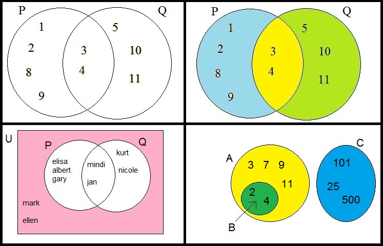
In figure 2 above, you see a few socalled "venn" diagrams, which helps explaining the "Union"
and "Intersection" of sets.

Suppose that P is the set {1,2,3,4,8,9}
You see that represented in figure 2, in the first quadrant, by a circle containing those elements.

Suppose that Q is the set {3,4,5,10,11}
You see that represented in figure 2, in the first quadrant too, by a second circle containing those elements.

- The Intersection of sets:

Now we might wonder: which elements do have "P" and "Q" in common?
From figure 2, it is obvious that these are the elements "3" and "4".
Those common elements are called the Intersection of the sets "P" and "Q".
It's notated in this way (using the example in figure 2), using the "⋂" symbol:

P ⋂ Q = {3,4}

In figure 2, the second quadrant, I represented the "Intersection" as the common (overlapped)
yellow area of the two circles.

- The Union of sets:

We can also "add" sets, or stated in "set theory" language, "join" sets or "union" sets.
In our example of P and Q above, the union would be {1,2,3,4,5,8,9,10,11}.
It's notated in this way (using the example in figure 2), using the "⋃" symbol:

P ⋃ Q = {1,2,3,4,5,8,9,10,11}

In figure 2, the second quadrant, I represented the "Union" as the combination of
both two circles (blue, yellow, and green area's).

Note: why don't we count an element like "3" double, that is, two times?
The elements themselves are fundamental. You can "draw" any closed line between any
number of elements, and thereby "declaring" a set.
This way, you might have multiple sets containing the same element. But not the elements themselves
will double magically. So, in Intersections or Unions we will count them one time.

- The complementary of a set, like Ā or A^C :

If we look at the example set P and Q again, and suppose we want to list
all elements which are not element of (or do not belong to) P, then in figure 2 (second quadrant),
it would be the green area, that is the elements {5,10,11}.

In general, if you have set "U", then the complementary set is often denoted by "U^C", or "Ū".

- Subsets:

In the fourth quadrant of figure 2, you see the sets A, B and C.
We can see that A, B, and C contain:

A={2,3,4,7,9,11}
B={2,4}
C={101,25,500}

It's crucial to note that the elements 2 and 4 belong to the set A as well.
Indeed, the circle representing A, contains all those elements as listed below.

By coincidence, B contains 2 and 4 as well (actually only 2 and 4).

As you might already have guessed, is the fact that B is a subset of A.
In contrast, if you take a look at P and Q again: in that case we do not have the situation
that either one is a full part of the other one.

In "set theory" language, if B is a subset of A, it is notated as:

B ⊂ A

- The Empty set ∅

As the last remark of this section, I like to attend you on the fact that set A is fully disconnected from set C.
They do no have any element in common. Their "intersection" is "empty", often denoted by the symbol "∅".
So, if sets do not have any intersection, we say that:

A ⋂ C = {∅}

Ok, now let's finally move on to "Probability calculus".

Chapter 5. Probability calculus.

When the subject is about "probability theory", usually, people speak of "events", and each of such an event
has a certain number of possible "outcomes", where each outcome has a certain "probability" to occur.

Actually, there are two main "forks" here:

1. The more "mundane" probability theory on a finite, and discrete number of possible outcomes of an experiment.
What I call "experiment" here, could be for example, the throwing of a dice, or drawing a card from a deck of cards,
or grabbing a ball from a large box with many differently coloured balls, or tossing a coin, etc.. etc..
Note that the "space" of all possible outcomes, is limited and contains discrete outcomes.
This collection of all possible outcomes is often also called sample space.
This is the subject of section 5.1.

2. We can also deal with a continuous stochastic variable.
This sounds more complex than it actually is. It simply means that the "space" of all possible outcomes, is continuous
and is "uncountable". For example, the position of a particle in space. In Quantum Mechanics, we may only speak of the
probability that a particle is in some region of space.
As another example, if you would measure the length of a very large group of people, the distrubution of the lengths
varies so much, that we may treat it as a continuous "variable".
This is the subject of section 5.2.

5.1 Probability theory of a discrete outcome space (sample space).

5.1.1 General Probability definition (Laplace).

As a simple but effective example: you can throw a dice (an event), and if you throw a six, then that is a certain outcome.
Ofcourse, in this case, there are 6 equivalent outcomes, which we can decribe with the set {1,2,3,4,5,6}.

In this example, we don't have to be like Einstein to formulate the "probability" of any of those outcomes.
Using plain logic: each number has a "one out of six" chance to occur.

So, for example, the probability of throwing a "3" (or any other face of the dice) is:

P(outcome=3) =

1 -- 6

For similar events, a "general equation" can be formulated. If there are N_f favourable outcomes
for a certain result "f", out of a total number of N_T outcomes, then the probability of finding "f" is:

P(f) =

Nf --       (equation 13) NT

Example:

The probability of drawing an "ace" from a deck of cards is:

P(ace) =

4 -- 52

Indeed, since there are 4 aces in the deck of 52 cards, the probability of finding some ace, must be 4/52.

Although we have not proven anything, here, all of the above calculations are simply based on "common sense".
Here are some other rather "logical" (but very important) theorems:

5.1.2 Some Theorems (without proof), and illustrative examples:

(1): Total of All Probabilities:

Consider an event with N possible (discrete) independent outcomes. Suppose that for outcome "i", the probability
is denoted by "P_i", then:

The Sum of all probabilities   =   Σ _i=1^i=N P_i   =   1       (equation 14)

As you know from former notes, the Σ is a shortcut notation for a summation of all P_i, where i runs from 1 to N.

Thus, for example, if you throw a dice, the total probability of throwing a 1, or 2, or 3, or 4
or 5, or 6, is "1". In other words, the probability of throwing whatever number, is "1".
So, you can sum up all individual probabilities and the full total just have to be "1".

(2): Complements rule:

It's universally true that:

If the probability on outcome "A" is P(A), then P(Not A) = 1 - P(A)       (equation 15)

Example:

Suppose you draw one card only, from a deck of cards.

Then the probability of drawing the "ace of spades", is 1/52.

So, finding NOT the ace of spades, is 1 - 1/52 = 52/52 - 1/52 = 51/52.

Example:

If you throw a dice once, then the probability of getting a "3" or "4" is: 1/6 + 1/6 = 2/6 = 1/3.

So, the probability of NOT getting a "3" or "4" is: 1 - 1/3 = 2/3.

(3): Adding probabilities:

This subject is not difficult, but it needs some "subtle" considerations.

The question is: how "much overlapping" exists between the event spaces (sample spaces), for which we want to
"add" the probabilities.
As you will see in a moment, not always can we simple add the individual probabilities "just like that".

We better view this from "set theory".

Case 1:

Suppose you (randomly) select an element from set A, and (randomly) select an element from set B.
Now if the intersection of A and B is empty or {∅}, then A and B have absolutely nothing in common.

The addition of probabilities is expressed in set language too. In this case, an event that applies to A
and an event that applies to B, is written as:

P(A ⋃ B) = P(A) + P(B)       (equation 16)

So, here we have a "pure" addition.

Case 2:

Again, suppose you (randomly) select an element from set A, and (randomly) select an element from set B.
Now if the intersection of A and B is NOT empty or {∅}, then A and B have elements in common.

To avoid "double counting" we must then "subtract" the intersection from the Sum of probabilities:

P(A ⋃ B) = P(A) + P(B) - P (A ⋂ B)       (equation 17)

Example of case 2:

Suppose you draw one card of a deck of cards.
What is the probability that this card is a "spade" or an "ace"?

There is an overlap between the set of all spades, and the set of all aces.
In other words: there exists an intersection between the set of all spades, and the set of all aces.
Namely, the card ace of spades.

Indeed, it's not always easy to take the right choice between using equation 15 or equation 16.
In this case, we were able to identify the intersection between the sets, so we must use equation 16.

So:

P(spades ⋃ ace) = P(spades) + P(ace) - P (spades ⋂ ace) = 13/52 + 4/52 - 1/52 = 16/52.

(4): Multiplying probabilities:

Again, there are several intracies here.

A proper treatment would go into the subject of "conditional" probabilities.
However, I will only touch the simplest case: when two (or more) events are completely independent.
If that is indeed so, you generally must multiply the individual probabilities of the events.

Example:

You toss a coin one time, and then throw a dice one time.
What is the probability of obtaining "tail" AND throwing a "3"?

These events are completely independent (let's not get philosophical).

So:

P(tail AND 3) = 1/2 x 1/6 = 1/12

Example:

You throw 2 times in row with a dice. What is the probability of throwing a "2" first, and a "3" the second time?

Again, these events are completely independent (let's not get philosophical).

So:

P("2" AND "3") = 1/6 x 1/6 = 1/36

It's sometimes not easy to decide if you must add probabilities like
in equations 15 or 16, or when you must multiply probabilities.
For what it's worth: Here is Albert's tip (not full proof):

-When in English you read: "event A" OR "event B": you probably (no pun intended) must add probabilities.
-When in English you read: "event A" AND "event B": you probably (no pun intended) must multiply probabilities.

5.1.3 The "Binomial Probability" equation.

Example:

If we throw a dice 3 times, we know how to calculate the probability to throw a "2" first, then a "5",
and then a "6". These are three independent "events", so we must multiply probabilities.

It will be this: P(2,5,6) = 1/6 x 1/6 x 1/6.

Now consider this: what is the probability to throw a "6" first, then a "6" again, then lastly, "NOT a 6"?

I suppose the answer is this: P(6,6,NOT 6) = 1/6 x 1/6 x 5/6.

Now take care: Suppose we call "p" the probability to throw a 6. Then throwing "NOT a 6" is "(1-p)".
Let's call (1-p)=q.

So, we can rewrite the probability above as: P(6,6,NOT 6) = p x p x (1-p) = p² x q.

Now, let's turn our attention to the "Binomial Probability" equation.

It's not unlike we have seen above. If we are dealing with "n" independent experiments (or events) where at each
event we can obtain "success/failure" or, equivalently, "yes/no", or whatever else two distinctive outcomes,
then the probability to find "k" successes in "n" experiments (or trials) is:

P(k) =

┌ n ┐ └ k ┘

pk (1-p)n-k       (equation 18)

Here, "p" is the probability to find "success" (or "yes", or other sort of twofold outcomes),
and (1-p) is the probability of "failure" (or "no", or other sort of twofold outcomes).

It's possible to proof equation 18, but I will only make it "plausible" here.

The term "p^k (1-p)^n-k" is actually not different then an extension of the example we saw above.

But why the "n choose k" term?

Well, we only ask for "k" successes out of "n" attempts.
Remember section 4.2? That section is titled "Combinations of "k" elements, from a larger set of "n" elements".

There we found that we can have "k" elements (successes) out of "n" elements (attempts), but there exists
a variety of the k's along the n's. For example, we can have "yyynnyynnnnnyy" with 7 "y's", but this one
"ynnnnyynnyynyy" has 7 "y's" too, so there are multiple Combinations of "k" elements, from a larger set of "n" elements.

So indeed, we have to multiply the factor "p^k (1-p)^n-k" with the "n choose k" term as well,
in order to find all combinations for which "p^k (1-p)^n-k" is true.

Task:
I have a task for you, if you like it. Google on the terms "Binomial Probability", and try to find some examples
with calculations. That's really instructive, since many folks have created rather nice examples.
Also, if you see nice documents, it's always good to see other prespectives as well.

5.2 Probability theory of continuous stochastic variable (sample space).

Ok, this is the last section of this very simple note.

Al of the above, dealt with a "discete" outcome space. However, in many occasions we have
a (nearly) continuous "outcome space".

-For example, the times when vistors enter a store.

-Or, the position of a particle on the x-axis (in 1 dim space). This might be considered to be really "continuous".

-Or, the length measured of 500000 people at the age of 30y.
In this case, the number of measurements is so large, that we may treat it as a continuous "variable".
Plotted in a XY graph, most measurements will be in the interval 140cm - 190cm, while the graph probably
will quickly lower at x > 190cm and x < 140cm.

Example:

Or, what about the lifetime of a lightbulb? Theoretically, the lifespan will be in the interval [0,∞],
but for a certain type, you might find a mean value of, say, 6 months.
Suppose you did an incredably large number of measurements. In a graph, you might find something like shown in figure 3:

Figure 3. lifetime of lightbulbs.



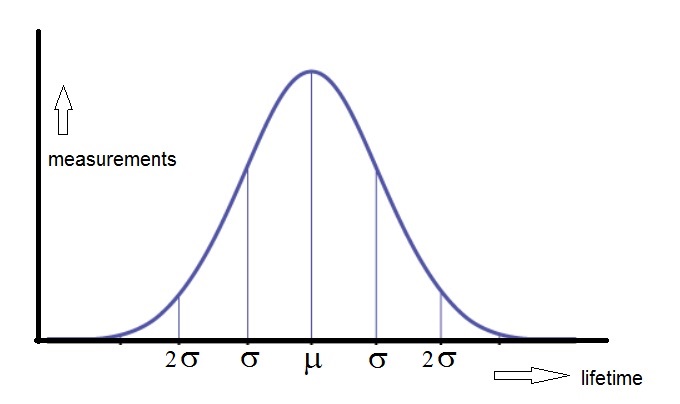
Most lightbulbs will obviously function with a lifespan near a certain mean value μ.
However, some will function for a very long time, much longer than μ, and ofcourse some
will function for a much shorter time.

This is all expressed in the example of figure 3. With graphs, usually, we talk about an "x-axis" and "y-axis".
But those are just names or conventions. In figure 3, we have the "livespan" having the role of "x",
and "number of measurements" having the role of "y".
Note that this particular figure is symmetrical around μ.

In case of a continuous stochastic variable, we have no other choice than to use a "probability function f(x)",
or more often called a "probability distribution".
When we see that in a graph, we see a continuous function in a XY coordinate system, where the "outcomes"
are on the x-axis, and the "frequency" is on the y-axis.

In former notes we already have seen that a definite integral is actually an infinite sum, where the
discreteness of the "intervals" goes to zero. See for example note 14.
We have a similar case here too.
Since the "total" probability must "add" up to "1", we have to use an definite integral over the full range of "x".

- Suppose that a "probability distribution" is completely defined over the interval x in [a,b], then:

∫_a^b f(x) dx = 1

Note that the sum (or integral) of the total probability corresponds to the "area" of the region bounded
by f(x) and the x-axis, over [a,b].

- Suppose that a "probability distribution" is defined over the interval x in [-∞,∞], then:

∫_-∞^∞ f(x) dx = 1

-Suppose that a "probability distribution" is defined over the interval x in [a,d], and we want
the probability of finding x in the interval [b,c], where a < b < c < d, then

P([b,c]) = ∫_b^c f(x) dx = F(c) - F(b)

Examples:

Example 1.

Suppose the probability distribution is f(x)=0.2.
This is an incredably simple function (it's a constant function: y is always 0.2, for all x).

In figure 4 below, you can see the function f(x)=0.2. Since, as a probability distribution, the total area must be "1",
the function then only can be meaningful over the interval x in [0,5].

Note that the area is defined by the rectangular region bounded by f(x) and the x-axis, for x in the interval [0,5].
So, the total area is 0.2 x 5 = 1, which is exactly what we expect to find.

Now, suppose we had the probability distribution is f(x)=0.5 instead. Then the x interval neccessarily had to be [0,2],
since the total probability always have to add up to "1".

Figure 4. Simple probability distribution defined by y=0.2.




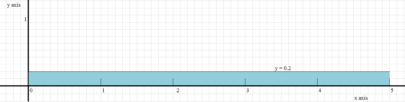
Question: what is the probability for x ≥ 4 (or 4 ≤ x ≤ 5)?

Answer:

P([4,5]) = ∫₄⁵ 0.2 dx = 0.2x|₄⁵ = 0.2 * 5 - 0.2 * 4 = 0.2

Take a look also at figure 4. Note that the total area is "1". Also note that you can devide
that area in 5 parts. One such part is defined by the interval 4 ≤ x ≤ 5, so that represents
an area of 1/5=0.2.

The "trick" to find the solution is ofcourse that you knew that the primitive function of f(x)=0.2,
is F(x)=0.2x.
For more information on primitives and definite integrals: see notes 8 and 14.

True, this example used a very simply probability function. However, the principle is the same,even if it's a horrible complex function.
You can calculate probabilities, as long as you can find the primitive function.

That's it. Hope you liked it !